Reinforcement Learning Applied in Automobile


Lane Detection and Lane Change

Reinforcement Learning Applied in Automobile

Choose Your Hands-on Learning Topic

Disclaimer

All software & hardware's used or referenced in this guide belong to their respective vendors. We have developed this guide based on our development infrastructure and this guide may or may not work on other systems and technical infrastructure. We are not liable for any direct or indirect problems caused to the users using this guide.

Executive Summary

The purpose of this document is to provide adequate information to users to implement a advanced reinforcement learning model. In order to achieve this, we are using the self driver car problem that may become a reality of automobile industries. The problem is be solved using Decision Trees, Random Forests a supervised machine learning model, Convolutional Neural Networks & Deep Q Networks.

Business Problem

Problem Statement

Identifying lanes on the road as performed by all human drivers to ensure their vehicles are within lane constraints when driving, so as to make sure traffic is smooth and minimize chances of collisions with other cars due to lane misalignment It is a critical task for an autonomous vehicle to perform. It turns out that recognizing lane markings on roads is possible using well known computer vision technique that avoids accidents & makes the traffic smooth. Lane Changing is an Important aspect of self-driving cars. Self-driving cars must incorporate lane changing system for smooth & efficient driving. For a self-driving cars When changing lanes, the most important thing is to wait until there is a clear gap in the traffic, then move safely and smoothly into the center of the desired lane, while maintaining space in the flow of traffic so that no other vehicle is forced to slow down, speed up, or change lanes to avoid collision.

Business Challenges

  • Accidents: Lane Changes Causes lot of accidents due to distracted drivers and driver error. Autonomous vehicles have great potential to dramatically reduce these numbers, not to mention save the economy from cost of injuries and lost work.
  • Winning Public and Individual trust : People the customers make comments like, “I would never trust technology enough to let it take over driving.” The fact is that sensors and properly configured machines can make faster, consistent, and emotion-free decisions than humans. In reality, not all accidents can be eliminated even with autonomous cars.
  • Continuous Technology and Standards Evolution : Technology is evolving into higher performing systems. It reaps benefits that occur from standards dictating acceptable levels of safety performance. Increase in the rate of development, Decrease in overall system cost per vehicle will occur with Well-drafted standards.

Business Context

Human driven cars are monitored by humans sitting behind a steering wheel. The driver of the car needs to be vary of variety of things. He/she needs to drive the vehicle with permissible speed, follow lane discipline etc. All these changes with the rapid development of complex technologies that slowly start to emerge on different cars is going to take over the various functions that were normally performed by the driver. The development of the technology directs us into the use of self-driving cars as well as driveless cars.

High Level Implementation Steps

Step 1 : Defining a Clear Problem Statement

Step 2 : Identification of the Input Data (Camera Images, Sensor Images)

Step 3 : Application of Computer Vision Techniques on the Input Road Image for Lane Detection or Identification

Step 4 : Once the Lane is Detected next step is to incorporate a lane changing system. So first the environment is downloaded & Started.

Step 5 : Once the Environment is initialized we need to examine the Observation & State Spaces

Step 6 : Training & test the agent on Action & States for a maximum reward using a Deep reinforcement algorithm called Deep Q Networks.

Model Selection

Model selection is the process of choosing between different machine learning, deep learning or reinforcement learning approaches - e.g. SVM, CNN, Deep Q Learning etc. or choosing between different hyperparameters or sets of features for the same machine/deep/reinforcement learning approach - e.g. deciding between the polynomial degrees/complexities for linear regression.

The choice of the actual learning algorithm is less important than you'd think - there may be a "best" algorithm for a particular problem, but often its performance is not much better than other well-performing approaches for that problem.

There may be certain qualities you look for in a model:

  • Interpretable - can we see or understand why the model is making the decisions it makes?
  • Simple - easy to explain and understand
  • Accurate
  • Fast (to train and test)
  • Scalable (it can be applied to a large dataset)

Our Problem here is a Reinforcement Learning Problem. The Problem is to identify lanes & drive the car along the identified lane with great steering control. There are various algorithms that could be used Ex: Q-Learning, State-Action-Reward-State-Action (SARSA), Deep Deterministic Policy Gradient (DDPG) etc. These could be alternative’s to DQN's. Below are the points makes Deep Q Networks an ideal choice.

  1. Q Learning are a powerful algorithm that helps the agent figure out exactly what action to perform. An environment with 10,000 states and 1,000 actions per state would create a table of 10 million cells. Then it happens that we can’t infer the Q-value of new states from already explored states because of the following reasons:
    • First, the amount of memory required to save and update that table would increase as the number of states increases
    • Second, the amount of time required to explore each state to create the required Q-table would be unrealistic.
  2. State-Action-Reward-State-Action (SARSA) resembles Q-Learning meaning to says it much much like Q-learning does, just that SARSA learns the Q-value based on the action performed by the current policy instead of the greedy policy.
  3. With Deep Deterministic Policy Gradient the action space is still discrete. Many tasks of interest, especially physical control tasks, the action space is continuous. If you discretize the action space too finely, you wind up having an action space that is too large.

With all the above being said Deep Q-learning (DQN) comes to our rescue, Deep Q Networks use a neural network to approximate the Q-value function. The state is given as the input and the Q-value of all possible actions is generated as the output. Given that our model input’s are images & videos with vehicles moving on the road, Neural networks with Convolution Networks Architecture perform really well gives the algorithm the possibility of maximizing the rewards based on the best policies employed.

What is Learning Algorithm?

  • A self-learning (not a human developed code) code, performs data analysis and extracts patterns (business characteristics) in data for business application development - a modern approach to application/software development.
  • Automatically understands and extracts data pattern a modern approach (change in business circumstance) and performs data analysis based on the new/changed data. - No code change required to implement changes that took place in the data (change in business)
Feature Engineering

Feature engineering is a crucial step in the process of predictive modeling. It involves the transformation of given feature space, typically using mathematical functions, with the objective of reducing the modeling error for a given target. However, there is no well-defined basis for performing effective feature engineering. It involves domain knowledge, intuition, and most of all, a lengthy process of trial and error. The human attention involved in overseeing this process significantly influences the cost of model generation. In this implementation we present a new framework to automate feature engineering. The Reinforcement model Deep Q-learning uses Neural Network architecture.

Feature engineering is the most important art in machine learning which creates a huge difference between a good model and a bad model.

Advantages of Feature Engineering

  • Good features provide you with the flexibility of choosing an algorithm; even if you choose a less complex model, you get good accuracy.
  • If you choose good features, then even simple ML algorithms do well.
  • Better features will lead you to better accuracy. You should spend more time on features engineering to generate the appropriate features for your dataset. If you derive the best and appropriate features, you have won most of the battle.
Data Management Lane Detection

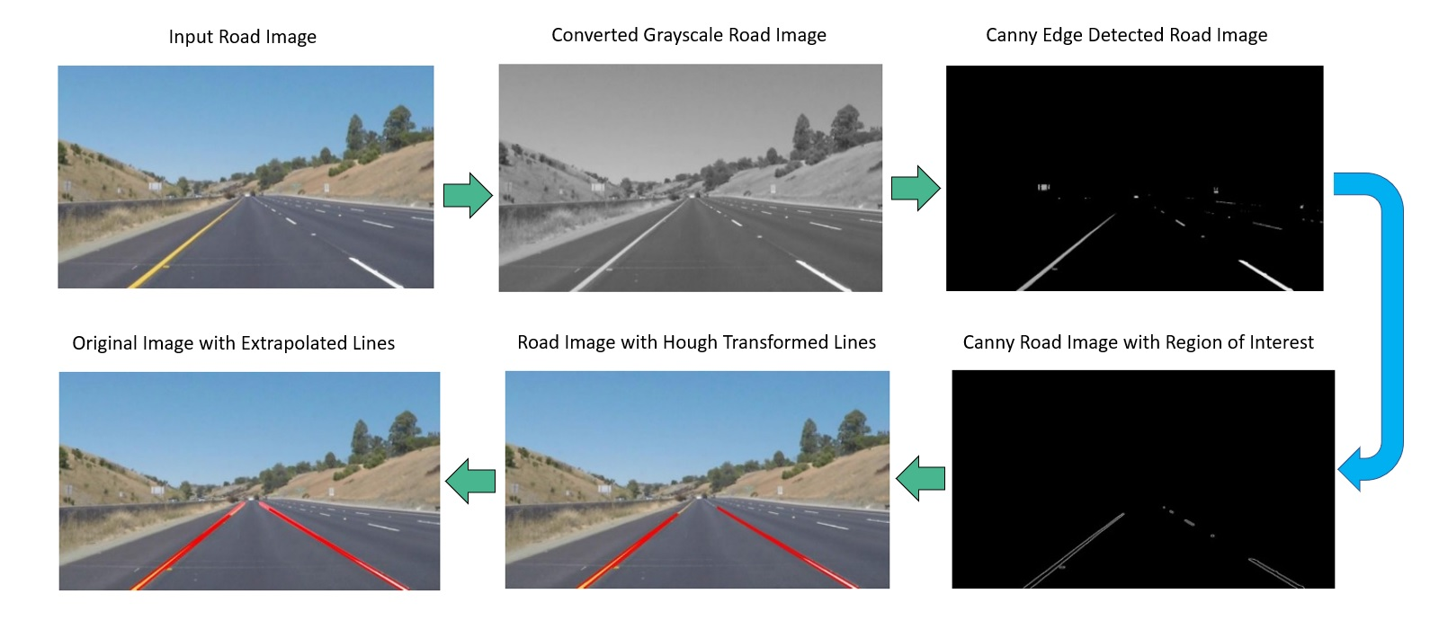
The Input Dataset are set of images that would undergo various computer vision techniques like color selection, region of interest selection, grayscaling, Gaussian smoothing, Canny Edge Detection and Hough Transform line detection. A pipeline is used to detect the line segments in the image, then average/extrapolate them and draw them onto the image for display.

What is the Input Data Set for Lane Detection?

The Input Dataset are set of images that would undergo various computer vision techniques. This is the actual data that is to under several computer vision techniques & finally detecting the lane lines.
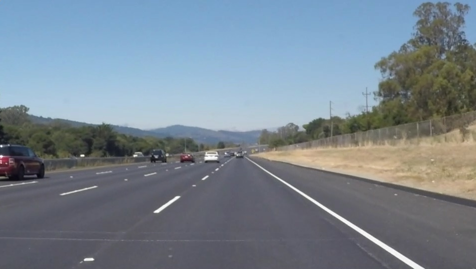
Data Management Lane Detection
Reinforcement Learning Libraries Used

There are several Reinforcement and data engineering libraries available. We are using the following libraries, and these libraries and their associated functions are readily available to use in Python to develop business application.

  • numpy 1.14.3
  • opencv 3.4.2
  • matplotlib 2.2.2
  • keras-rl 0..4.2

Classifier/Model Used

As we explained we are using Reinforcement learning model Deep Neural Networks (DQN).

  • Deep Neural Networks
  • Deep Q-Learning

Model Building Blocks

There are several technical and functional components involved in implementing this model. Here are the key building blocks to implement the model.
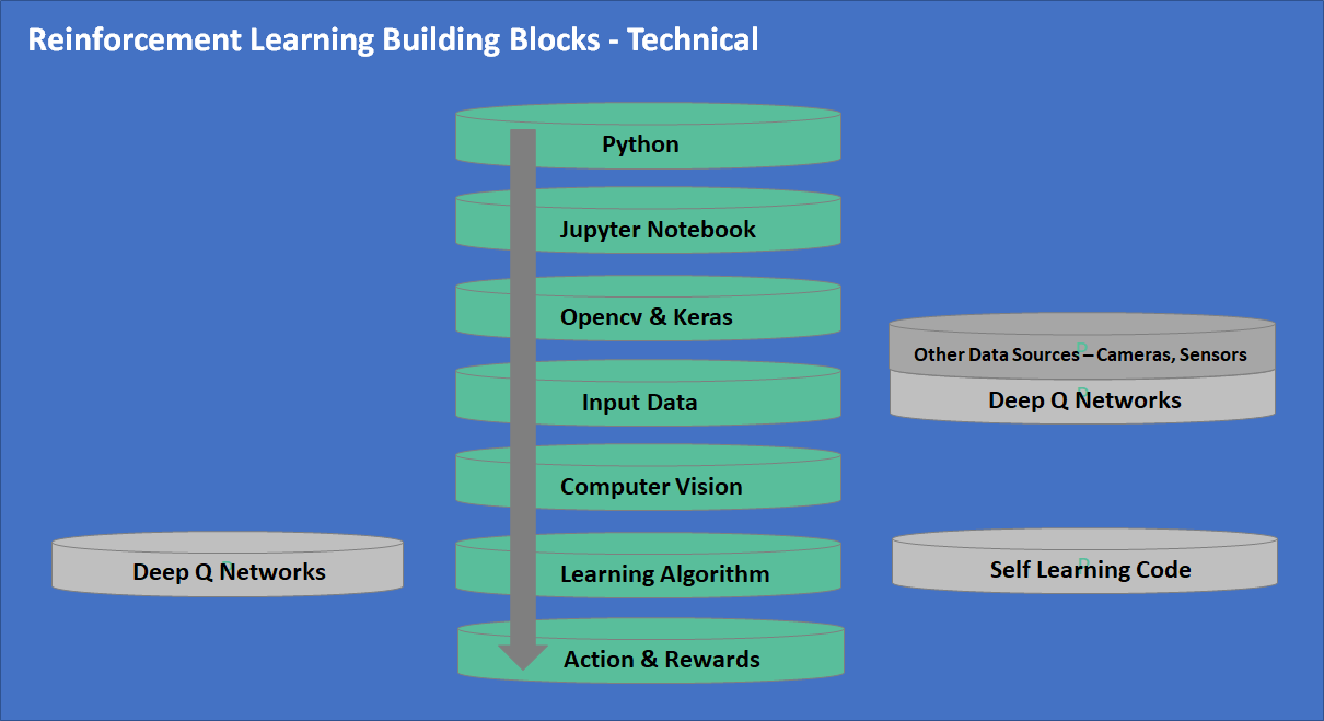
Model Building Blocks

Model Building Implementation Steps

A model implementation, to address a given problem involves several steps. Here are the key steps that are involved to implement a model. You can customize these steps as needed and we developed these steps for learning purpose only.
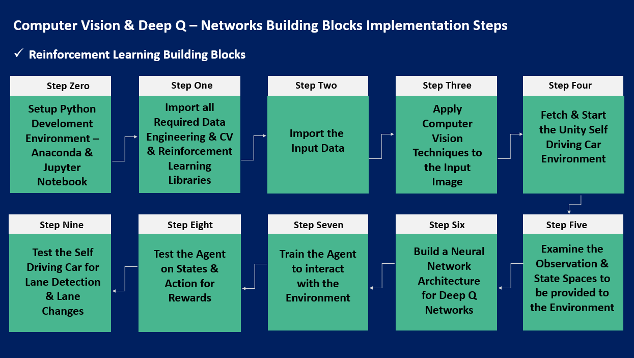
Model Building Implementation Steps
Model Implementation Code Block

  • # Step 0- Import the Data Source Path
    # Our Implementation Approach follows importing the Input Data, Training Data & Test Data from local hard drive.
    # As we don't want to hard code the Data source path, we use .INI(Configuration file) for getting the file paths.
    # The Library used for this is OS.
    import os
    vAR_INI_PATH = os.environ.get('AI_SELF_DRIVEN_CAR')
    import configparser
    vAR_Config = configparser.ConfigParser(allow_no_value=True)
    vAR_Config.read(vAR_INI_PATH)
    vAR_Data = vAR_Config.sections()
    vAR_Config.sections()
    vAR_Lane_Detection_Input_Image_Path = vAR_Config['Data Source Path']['LANE_DETECTION_IMAGE_INPUT_PATH']
    vAR_Lane_Change_Simulator_Path = vAR_Config['Data Source Path']['LANE_CHANGE_SIMULATOR_PATH']
  • # Step 1- Import the Required Libraries
    import cv2
    import numpy as vAR_np
    import matplotlib.pyplot as vAR_plt
  • # Step 2- Import the Input Data
    vAR_image = cv2.imread(vAR_Lane_Detection_Input_Image_Path)
  • # Step 3- Applying the Necessary Computer Vision Technique to the Input Road Image from the Camera
    ## Canny Edge Detection
    def vAR_Canny(vAR_image):
    vAR_gray= cv2.cvtColor(vAR_image,cv2.COLOR_RGB2GRAY)
    vAR_blur = cv2.GaussianBlur(vAR_gray,(5,5),0)
    vAR_canny = cv2.Canny(vAR_blur,50,150)
    return vAR_Canny
    ### Finding the Region of Interest in the Canned Image -
    def vAR_Region_of_Interest(vAR_image):
    vAR_height = vAR_image.shape[0]
    vAR_polygons = vAR_np.array([
    [(200,vAR_height),(1100,vAR_height),(550,250)]
    ])
    vAR_mask = vAR_np.zeros_like(vAR_image)
    cv2.fillPoly(vAR_mask,vAR_polygons,255)
    vAR_masked_image = cv2.bitwise_and(vAR_image,vAR_mask) #
    return vAR_masked_image
    def vAR_display_lines(vAR_image, vAR_lines):
    vAR_line_image = vAR_np.zeros_like(vAR_image)
    if vAR_lines is not None:
    for vAR_line in vAR_lines:
    #print(vAR_line)
    vAR_x1, vAR_y1, vAR_x2, vAR_y2 = vAR_line.reshape(4)
    cv2.line(vAR_line_image,(vAR_x1, vAR_y1),(vAR_x2, vAR_y2), (255,0,0), 10)
    return vAR_line_image
    vAR_image = cv2.imread(vAR_Lane_Detection_Input_Image_Path)
    vAR_lane_image = vAR_np.copy(vAR_image)
    vAR_gray= cv2.cvtColor(vAR_lane_image,cv2.COLOR_RGB2GRAY)
    vAR_blur = cv2.GaussianBlur(vAR_gray,(5,5),0)
    vAR_canny_image = cv2.Canny(vAR_blur,50,150)
    vAR_cropped_image = vAR_Region_of_Interest(vAR_canny_image)
    vAR_lines = cv2.HoughLinesP(vAR_cropped_image, 2, vAR_np.pi/180, 100, vAR_np.array([]), minLineLength=40, maxLineGap=5)
    #vAR_averaged_lines = vAR_average_slope_intercept(vAR_lane_image, vAR_lines)
    vAR_line_image = vAR_display_lines(vAR_lane_image, vAR_lines)
    vAR_combo_image = cv2.addWeighted(vAR_lane_image, 0.8, vAR_line_image, 1, 1)
    #vAR_plt.imshow(vAR_canny)
    #vAR_plt.show()
    cv2.imshow("vAR_result",vAR_combo_image)
    cv2.waitKey(0)
    import random
    import datetime
    import os
    import time
    import matplotlib.pyplot as vAR_plt
    from mlagents.envs import UnityEnvironment
    %matplotlib inline
  • # Step 4- Fetch & Start the Unity Self – driving Environment
    vAR_env = vAR_Lane_Change_Simulator_Path
    vAR_train_mode = True # Whether to run the environment in training or inference mode
    vAR_env = UnityEnvironment(file_name=vAR_env, worker_id= 3)
    # Set the default brain to work with
    vAR_default_brain = vAR_env.brain_names[0]
    vAR_brain = vAR_env.brains[vAR_default_brain]
  • # Step 5 – Examine Observation & State spaces for the Environment
    vAR_env_info = vAR_env.reset(train_mode=vAR_train_mode)[vAR_default_brain]
    # Examine the state space for the default brain
    print("Agent state looks like: \n{}".format(vAR_env_info.vector_observations[0]))
    # Examine the observation space for the default brain
    for vAR_observation in vAR_env_info.visual_observations:
    print("Agent observations look like:")
    if vAR_observation.shape[3] == 3:
    vAR_plt.imshow(vAR_observation[0,:,:,:])
    else:
    vAR_plt.imshow(vAR_observation[0,:,:,0])
    # Set Parameters
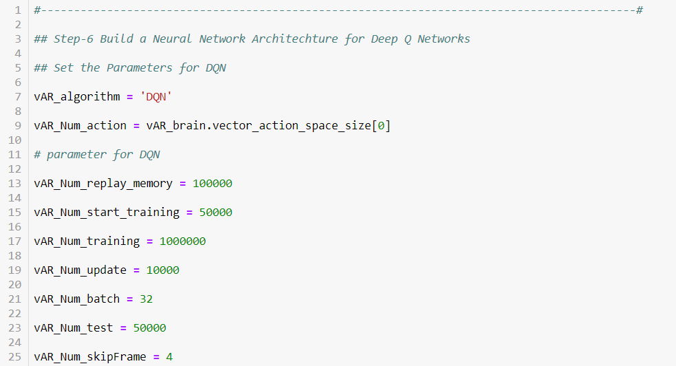
    vAR_algorithm = 'DQN'
    vAR_Num_action = vAR_brain.vector_action_space_size[0]
    # parameter for DQN
    vAR_Num_replay_memory = 100000
    vAR_Num_start_training = 50000
    vAR_Num_training = 1000000
    vAR_Num_update = 10000
    vAR_Num_batch = 32
    vAR_Num_test = 50000
    vAR_Num_skipFrame = 4
    vAR_Num_stackFrame = 4
    vAR_Num_colorChannel = 1
    vAR_Num_obs = len(vAR_env_info.visual_observations)
    vAR_Epsilon = 1.0
    vAR_Final_epsilon = 0.1
    vAR_Gamma = 0.99
    vAR_Learning_rate = 0.00025
    # Parameter for LSTM
    vAR_Num_dataSize = 366
    vAR_Num_cellState = 512
    # Parameters for network
    vAR_img_size = 80
    vAR_sensor_size = 360
    vAR_first_conv = [8,8,vAR_Num_colorChannel * vAR_Num_stackFrame * vAR_Num_obs,32]
    vAR_second_conv = [4,4,32,64]
    vAR_third_conv = [3,3,64,64]
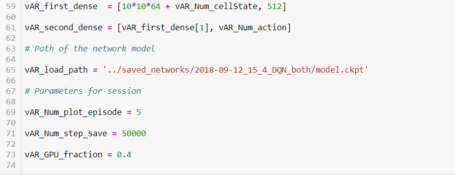
    vAR_first_dense = [10*10*64 + vAR_Num_cellState, 512]
    vAR_second_dense = [vAR_first_dense[1], vAR_Num_action]
    # Path of the network model
    vAR_load_path = '../saved_networks/2018-09-12_15_4_DQN_both/model.ckpt'
    # Parameters for session
    vAR_Num_plot_episode = 5
    vAR_Num_step_save = 50000
    vAR_GPU_fraction = 0.4
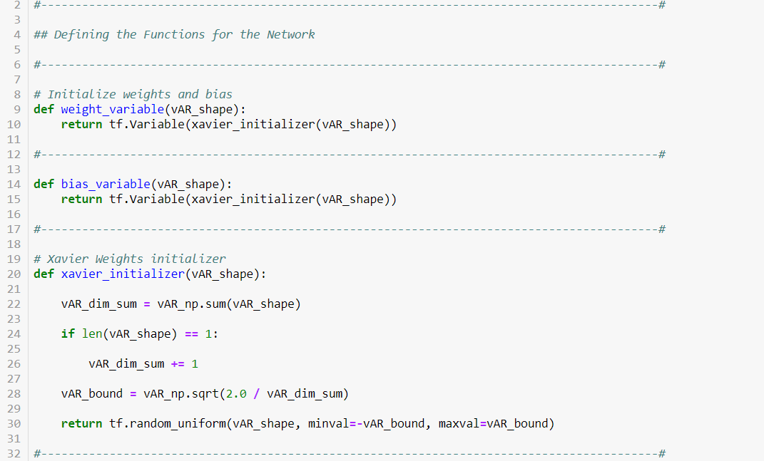
    # Initialize weights and bias
    def weight_variable(vAR_shape):
    return tf.Variable(xavier_initializer(vAR_shape))
    def bias_variable(vAR_shape):
    return tf.Variable(xavier_initializer(vAR_shape))
    # Xavier Weights initializer
    def xavier_initializer(vAR_shape):
    vAR_dim_sum = vAR_np.sum(vAR_shape)
    if len(vAR_shape) == 1:
    vAR_dim_sum += 1
    vAR_bound = vAR_np.sqrt(2.0 / vAR_dim_sum)
    return tf.random_uniform(vAR_shape, minval=-vAR_bound, maxval=vAR_bound)
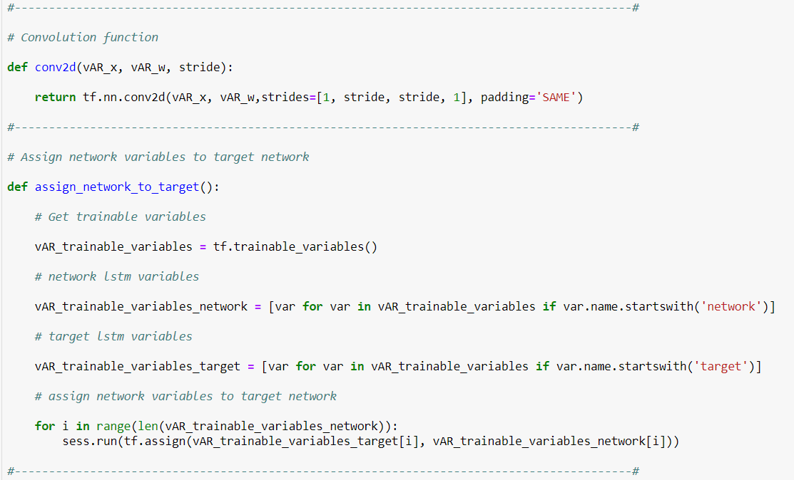
    # Convolution function
    def conv2d(vAR_x, vAR_w, stride):
    return tf.nn.conv2d(vAR_x, vAR_w,strides=[1, stride, stride, 1], padding='SAME')
    # Assign network variables to target network
    def assign_network_to_target():
    # Get trainable variables
    vAR_trainable_variables = tf.trainable_variables()
    # network lstm variables
    vAR_trainable_variables_network = [var for var in vAR_trainable_variables if var.name.startswith('network')]
    # target lstm variables
    vAR_trainable_variables_target = [var for var in vAR_trainable_variables if var.name.startswith('target')]
    # assign network variables to target network
    for i in range(len(vAR_trainable_variables_network)):
    sess.run(tf.assign(vAR_trainable_variables_target[i], vAR_trainable_variables_network[i]))
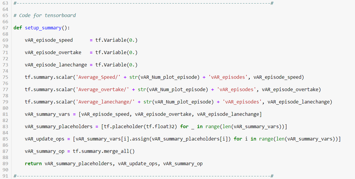
    # Code for tensorboard
    def setup_summary():
    vAR_episode_speed = tf.Variable(0.)
    vAR_episode_overtake = tf.Variable(0.)
    vAR_episode_lanechange = tf.Variable(0.)
    tf.summary.scalar('Average_Speed/' + str(vAR_Num_plot_episode) + 'vAR_episodes', vAR_episode_speed)
    tf.summary.scalar('Average_overtake/' + str(vAR_Num_plot_episode) + 'vAR_episodes', vAR_episode_overtake)
    tf.summary.scalar('Average_lanechange/' + str(vAR_Num_plot_episode) + 'vAR_episodes', vAR_episode_lanechange)
    vAR_summary_vars = [vAR_episode_speed, vAR_episode_overtake, vAR_episode_lanechange]
    vAR_summary_placeholders = [tf.placeholder(tf.float32) for _ in range(len(vAR_summary_vars))]
    vAR_update_ops = [vAR_summary_vars[i].assign(vAR_summary_placeholders[i]) for i in range(len(vAR_summary_vars))]
    vAR_summary_op = tf.summary.merge_all()
    return vAR_summary_placeholders, vAR_update_ops, vAR_summary_op
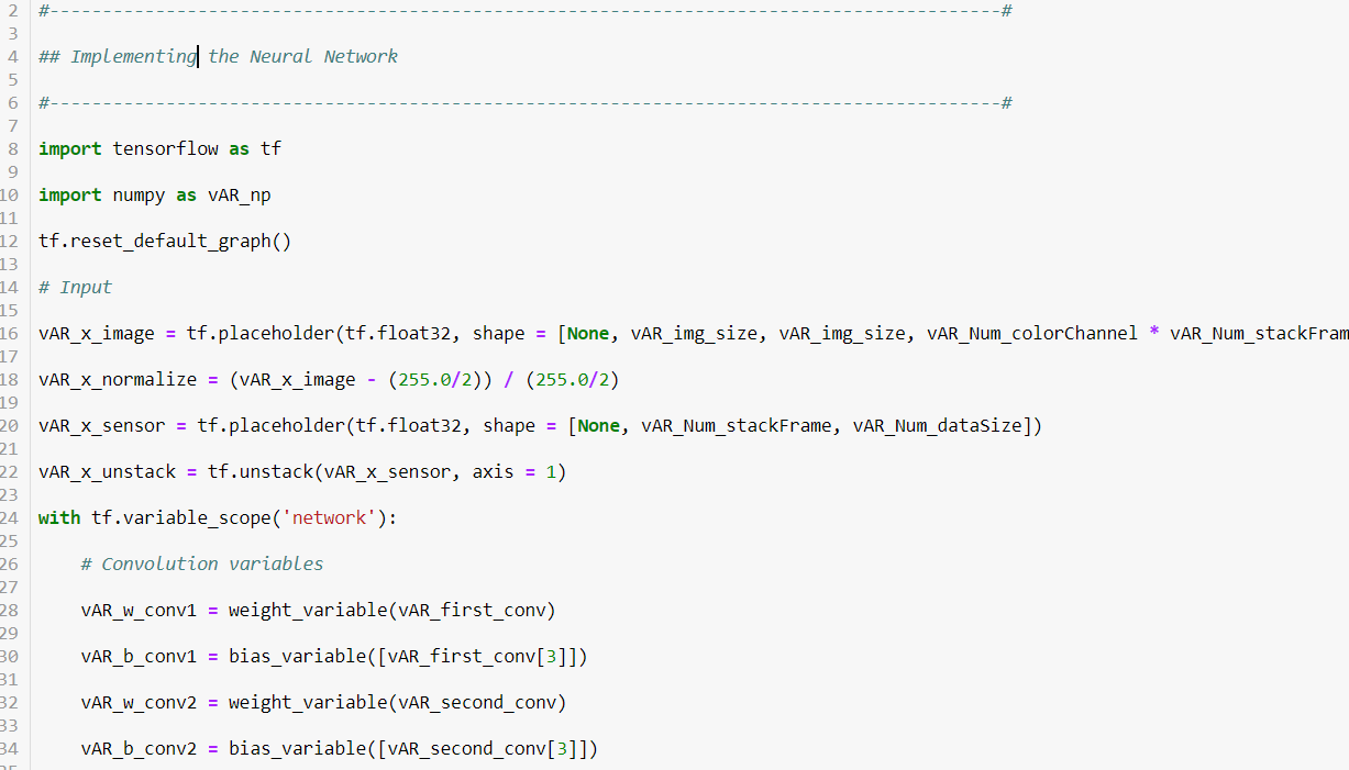
  • # Step 6 – Build a Neural Network Architecture
    import tensorflow as tf
    import numpy as vAR_np
    tf.reset_default_graph()
    # Input
    vAR_x_image = tf.placeholder(tf.float32, shape = [None, vAR_img_size, vAR_img_size, vAR_Num_colorChannel * vAR_Num_stackFrame * vAR_Num_obs])
    vAR_x_normalize = (vAR_x_image - (255.0/2)) / (255.0/2)
    vAR_x_sensor = tf.placeholder(tf.float32, shape = [None, vAR_Num_stackFrame, vAR_Num_dataSize])
    vAR_x_unstack = tf.unstack(vAR_x_sensor, axis = 1)
    with tf.variable_scope('network'):
    # Convolution variables
    vAR_w_conv1 = weight_variable(vAR_first_conv)
    vAR_b_conv1 = bias_variable([vAR_first_conv[3]])
    vAR_w_conv2 = weight_variable(vAR_second_conv)
    vAR_b_conv2 = bias_variable([vAR_second_conv[3]])
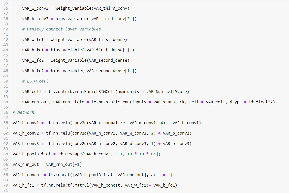
    vAR_w_conv3 = weight_variable(vAR_third_conv)
    vAR_b_conv3 = bias_variable([vAR_third_conv[3]])
    # Densely connect layer variables
    vAR_w_fc1 = weight_variable(vAR_first_dense)
    vAR_b_fc1 = bias_variable([vAR_first_dense[1]])
    vAR_w_fc2 = weight_variable(vAR_second_dense)
    vAR_b_fc2 = bias_variable([vAR_second_dense[1]])
    # LSTM cell
    vAR_cell = tf.contrib.rnn.BasicLSTMCell(num_units = vAR_Num_cellState)
    vAR_rnn_out, vAR_rnn_state = tf.nn.static_rnn(inputs = vAR_x_unstack, cell = vAR_cell, dtype = tf.float32)
    # Network
    vAR_h_conv1 = tf.nn.relu(conv2d(vAR_x_normalize, vAR_w_conv1, 4) + vAR_b_conv1)
    vAR_h_conv2 = tf.nn.relu(conv2d(vAR_h_conv1, vAR_w_conv2, 2) + vAR_b_conv2)
    vAR_h_conv3 = tf.nn.relu(conv2d(vAR_h_conv2, vAR_w_conv3, 1) + vAR_b_conv3)
    vAR_h_pool3_flat = tf.reshape(vAR_h_conv3, [-1, 10 * 10 * 64])
    vAR_rnn_out = vAR_rnn_out[-1]
    vAR_h_concat = tf.concat([vAR_h_pool3_flat, vAR_rnn_out], axis = 1)
    vAR_h_fc1 = tf.nn.relu(tf.matmul(vAR_h_concat, vAR_w_fc1)+ vAR_b_fc1)
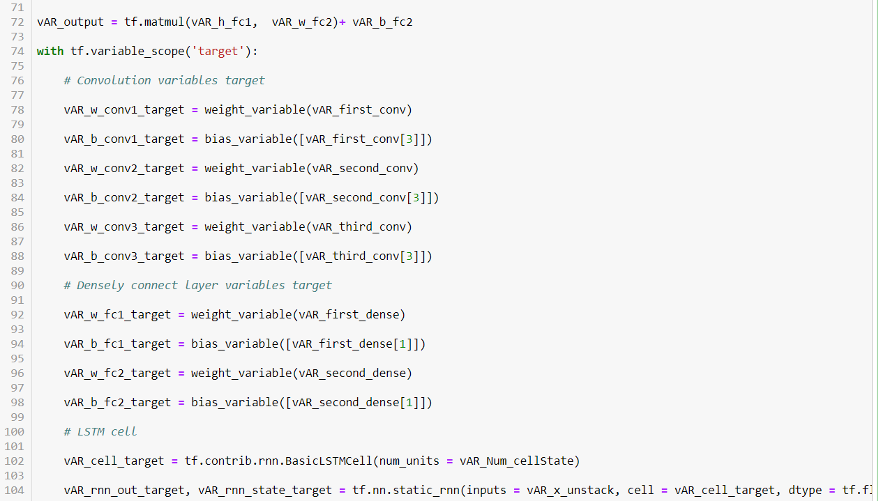
    vAR_output = tf.matmul(vAR_h_fc1, vAR_w_fc2)+ vAR_b_fc2
    with tf.variable_scope('target'):
    # Convolution variables target
    vAR_w_conv1_target = weight_variable(vAR_first_conv)
    vAR_b_conv1_target = bias_variable([vAR_first_conv[3]])
    vAR_w_conv2_target = weight_variable(vAR_second_conv)
    vAR_b_conv2_target = bias_variable([vAR_second_conv[3]])
    vAR_w_conv3_target = weight_variable(vAR_third_conv)
    vAR_b_conv3_target = bias_variable([vAR_third_conv[3]])
    # Densely connect layer variables target
    vAR_w_fc1_target = weight_variable(vAR_first_dense)
    vAR_b_fc1_target = bias_variable([vAR_first_dense[1]])
    vAR_w_fc2_target = weight_variable(vAR_second_dense)
    vAR_b_fc2_target = bias_variable([vAR_second_dense[1]])
    # LSTM cell
    vAR_cell_target = tf.contrib.rnn.BasicLSTMCell(num_units = vAR_Num_cellState)
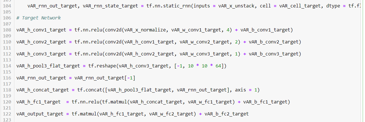
    vAR_rnn_out_target, vAR_rnn_state_target = tf.nn.static_rnn(inputs = vAR_x_unstack, cell = vAR_cell_target, dtype = tf.float32)
    # Target Network
    vAR_h_conv1_target = tf.nn.relu(conv2d(vAR_x_normalize, vAR_w_conv1_target, 4) + vAR_b_conv1_target)
    vAR_h_conv2_target = tf.nn.relu(conv2d(vAR_h_conv1_target, vAR_w_conv2_target, 2) + vAR_b_conv2_target)
    vAR_h_conv3_target = tf.nn.relu(conv2d(vAR_h_conv2_target, vAR_w_conv3_target, 1) + vAR_b_conv3_target)
    vAR_h_pool3_flat_target = tf.reshape(vAR_h_conv3_target, [-1, 10 * 10 * 64])
    vAR_rnn_out_target = vAR_rnn_out_target[-1]
    vAR_h_concat_target = tf.concat([vAR_h_pool3_flat_target, vAR_rnn_out_target], axis = 1)
    vAR_h_fc1_target = tf.nn.relu(tf.matmul(vAR_h_concat_target, vAR_w_fc1_target) + vAR_b_fc1_target)
    vAR_output_target = tf.matmul(vAR_h_fc1_target, vAR_w_fc2_target) + vAR_b_fc2_target
    ## Loss & Train
    vAR_action_target = tf.placeholder(tf.float32, shape = [None, vAR_Num_action])
    vAR_y_target = tf.placeholder(tf.float32, shape = [None])
    vAR_y_prediction = tf.reduce_sum(tf.multiply(vAR_output, vAR_action_target), reduction_indices = 1)
    vAR_Loss = tf.reduce_mean(tf.square(vAR_y_prediction - vAR_y_target))
    vAR_train_step = tf.train.AdamOptimizer(learning_rate = vAR_Learning_rate, epsilon = 1e-02).minimize(vAR_Loss)
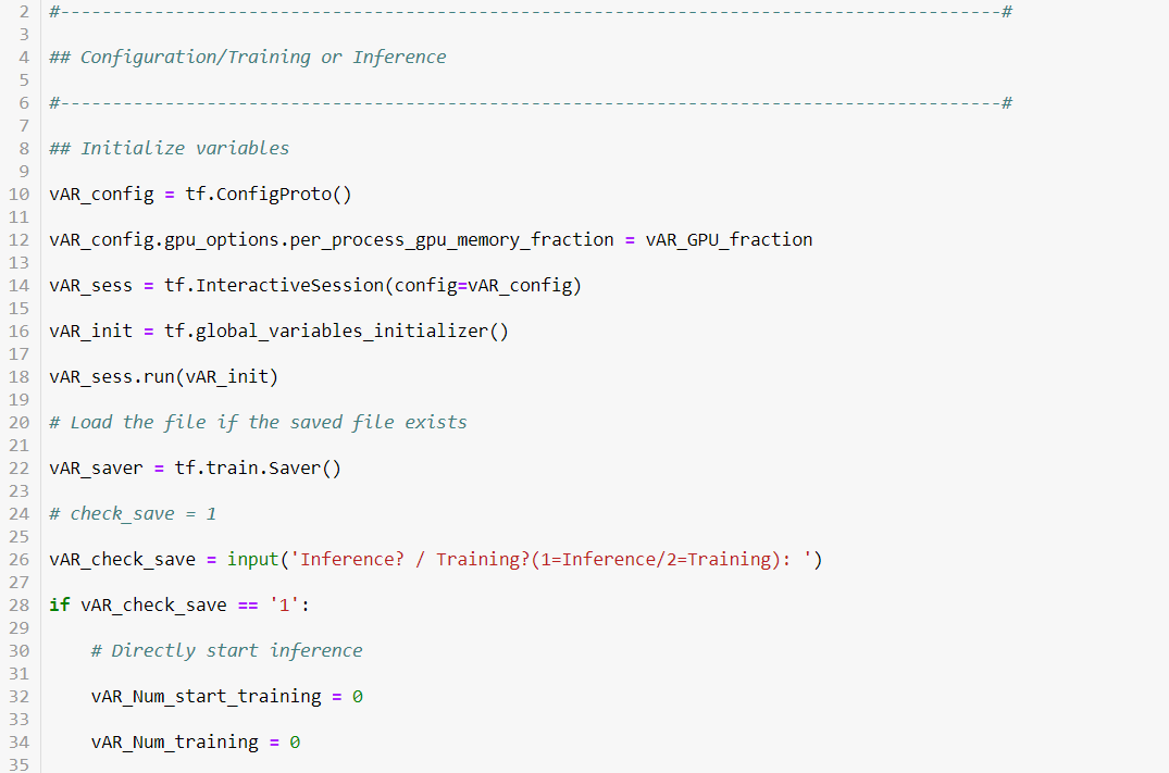
    ## Initialize variables
    vAR_config = tf.ConfigProto()
    vAR_config.gpu_options.per_process_gpu_memory_fraction = vAR_GPU_fraction
    vAR_sess = tf.InteractiveSession(config=vAR_config)
    vAR_init = tf.global_variables_initializer()
    vAR_sess.run(vAR_init)
    # Load the file if the saved file exists
    vAR_saver = tf.train.Saver()
    # check_save = 1
    vAR_check_save = input('Inference? / Training?(1=Inference/2=Training): ')
    if vAR_check_save == '1':
    # Directly start inference
    vAR_Num_start_training = 0
    vAR_Num_training = 0
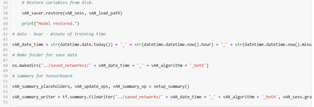
    # Restore variables from disk.
    vAR_saver.restore(vAR_sess, vAR_load_path)
    print("Model restored.")
    # date - hour - minute of training time
    vAR_date_time = str(datetime.date.today()) + '_' + str(datetime.datetime.now().hour) + '_' + str(datetime.datetime.now().minute)
    # Make folder for save data
    os.makedirs('../saved_networks1/' + vAR_date_time + '_' + vAR_algorithm + '_both')
    # Summary for tensorboard
    vAR_summary_placeholders, vAR_update_ops, vAR_summary_op = setup_summary()
    vAR_summary_writer = tf.summary.FileWriter('../saved_networks/' + vAR_date_time + '_' + vAR_algorithm + '_both', vAR_sess.graph)
    ## Functions for Training
    # Initialize input
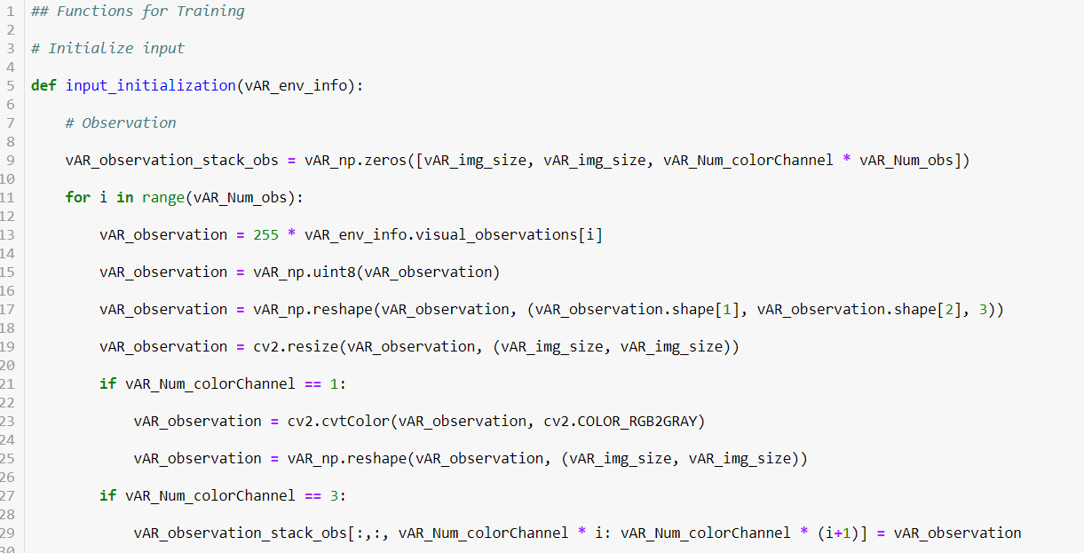
    def input_initialization(vAR_env_info):
    # Observation
    vAR_observation_stack_obs = vAR_np.zeros([vAR_img_size, vAR_img_size, vAR_Num_colorChannel * vAR_Num_obs])
    for i in range(vAR_Num_obs):
    vAR_observation = 255 * vAR_env_info.visual_observations[i]
    vAR_observation = vAR_np.uint8(vAR_observation)
    vAR_observation = vAR_np.reshape(vAR_observation, (vAR_observation.shape[1], vAR_observation.shape[2], 3))
    vAR_observation = cv2.resize(vAR_observation, (vAR_img_size, vAR_img_size))
    if vAR_Num_colorChannel == 1:
    vAR_observation = cv2.cvtColor(vAR_observation, cv2.COLOR_RGB2GRAY)
    vAR_observation = vAR_np.reshape(vAR_observation, (vAR_img_size, vAR_img_size))
    if vAR_Num_colorChannel == 3:
    vAR_observation_stack_obs[:,:, vAR_Num_colorChannel * i: vAR_Num_colorChannel * (i+1)] = vAR_observation
    else:
    vAR_observation_stack_obs[:,:, i] = vAR_observation
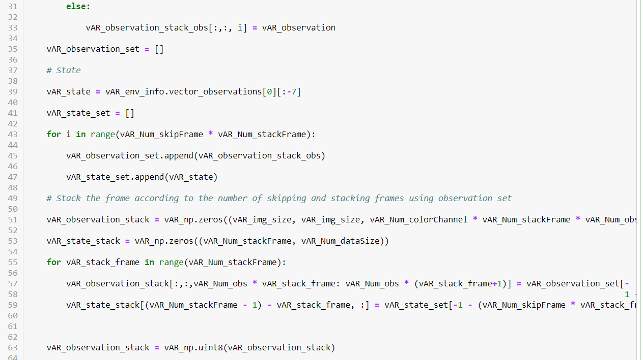
    vAR_observation_set = []
    # State
    vAR_state = vAR_env_info.vector_observations[0][:-7]
    vAR_state_set = []
    for i in range(vAR_Num_skipFrame * vAR_Num_stackFrame):
    vAR_observation_set.append(vAR_observation_stack_obs)
    vAR_state_set.append(vAR_state)
    # Stack the frame according to the number of skipping and stacking frames using observation set
    vAR_observation_stack = vAR_np.zeros((vAR_img_size, vAR_img_size, vAR_Num_colorChannel * vAR_Num_stackFrame * vAR_Num_obs))
    vAR_state_stack = vAR_np.zeros((vAR_Num_stackFrame, vAR_Num_dataSize))
    for vAR_stack_frame in range(vAR_Num_stackFrame):
    vAR_observation_stack[:,:,vAR_Num_obs * vAR_stack_frame: vAR_Num_obs * (vAR_stack_frame+1)] = vAR_observation_set[-
    1 - (vAR_Num_skipFrame * vAR_stack_frame)]
    vAR_state_stack[(vAR_Num_stackFrame - 1) - vAR_stack_frame, :] = vAR_state_set[-1 - (vAR_Num_skipFrame * vAR_stack_frame)]
    vAR_observation_stack = vAR_np.uint8(vAR_observation_stack)
    vAR_state_stack = vAR_np.uint8(vAR_state_stack)
    return vAR_observation_stack, vAR_observation_set, vAR_state_stack, vAR_state_set
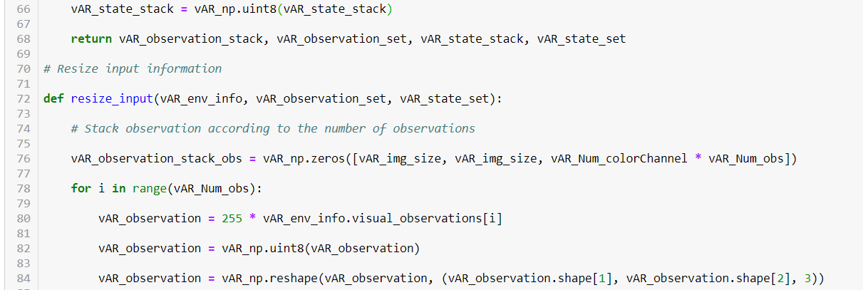
    # Resize input information
    def resize_input(vAR_env_info, vAR_observation_set, vAR_state_set):
    # Stack observation according to the number of observations
    vAR_observation_stack_obs = vAR_np.zeros([vAR_img_size, vAR_img_size, vAR_Num_colorChannel * vAR_Num_obs])
    for i in range(vAR_Num_obs):
    vAR_observation = 255 * vAR_env_info.visual_observations[i]
    vAR_observation = vAR_np.uint8(vAR_observation)
    vAR_observation = vAR_np.reshape(vAR_observation, (vAR_observation.shape[1], vAR_observation.shape[2], 3))
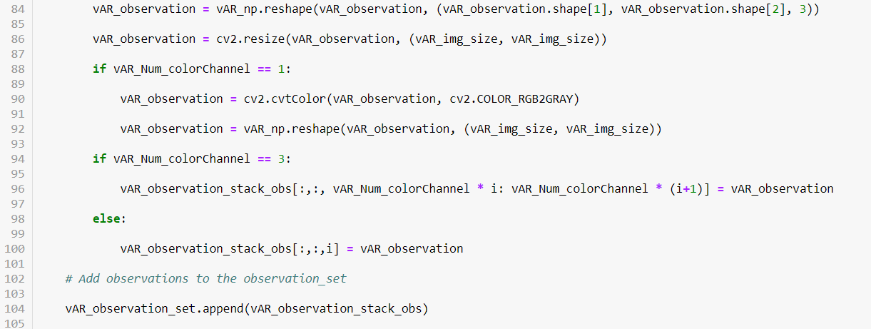
    vAR_observation = cv2.resize(vAR_observation, (vAR_img_size, vAR_img_size))
    if vAR_Num_colorChannel == 1:
    vAR_observation = cv2.cvtColor(vAR_observation, cv2.COLOR_RGB2GRAY)
    vAR_observation = vAR_np.reshape(vAR_observation, (vAR_img_size, vAR_img_size))
    if vAR_Num_colorChannel == 3:
    vAR_observation_stack_obs[:,:, vAR_Num_colorChannel * i: vAR_Num_colorChannel * (i+1)] = vAR_observation
    else:
    vAR_observation_stack_obs[:,:,i] = vAR_observation
    # Add observations to the observation_set
    vAR_observation_set.append(vAR_observ0ation_stack_obs)
    # State
    vAR_state = vAR_env_info.vector_observations[0][:-7]
    # Add state to the state_set
    vAR_state_set.append(vAR_state)
    # Stack the frame according to the number of skipping and stacking frames using observation set
    vAR_observation_stack = vAR_np.zeros((vAR_img_size, vAR_img_size, vAR_Num_colorChannel * vAR_Num_stackFrame * vAR_Num_obs))
    vAR_state_stack = vAR_np.zeros((vAR_Num_stackFrame, vAR_Num_dataSize))
    for vAR_stack_frame in range(vAR_Num_stackFrame):
    vAR_observation_stack[:,:,vAR_Num_obs * vAR_stack_frame: vAR_Num_obs * (vAR_stack_frame+1)] = vAR_observation_set[-1 - (vAR_Num_skipFrame * vAR_stack_frame)]
    vAR_state_stack[(vAR_Num_stackFrame - 1) - vAR_stack_frame, :] = vAR_state_set[-1 - (vAR_Num_skipFrame * vAR_stack_frame)]
    del vAR_observation_set[0]
    del vAR_state_set[0]
    vAR_observation_stack = vAR_np.uint8(vAR_observation_stack)
    vAR_state_stack = vAR_np.uint8(vAR_state_stack)
    return vAR_observation_stack, vAR_observation_set, vAR_state_stack, vAR_state_set
    # Get progress according to the number of steps
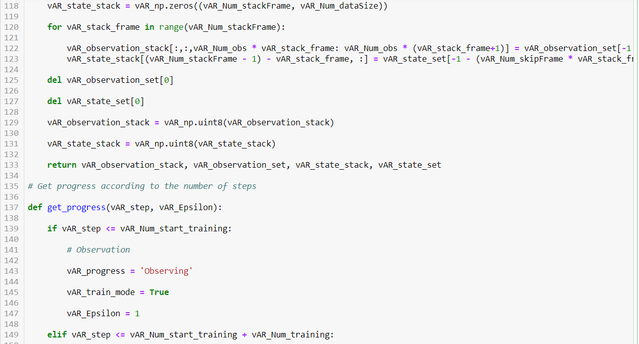
    def get_progress(vAR_step, vAR_Epsilon):
    if vAR_step <= vAR_Num_start_training:
    # Observation
    vAR_progress = 'Observing'
    vAR_train_mode = True
    vAR_Epsilon = 1
    elif vAR_step <= vAR_Num_start_training + vAR_Num_training:
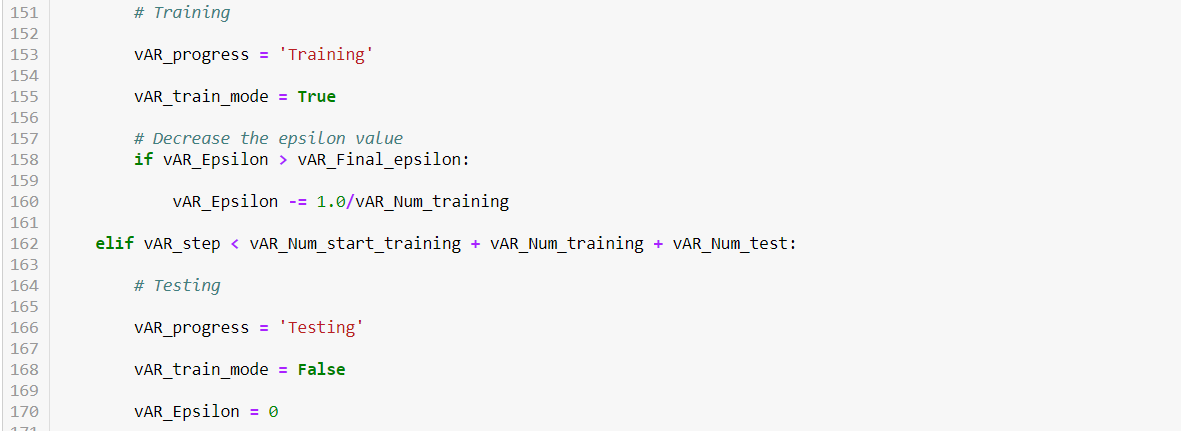
  • # Step 7 – Training the Agent
    # Training
    vAR_progress = 'Training'
    vAR_train_mode = True
    # Decrease the epsilon value
    if vAR_Epsilon > vAR_Final_epsilon:
    vAR_Epsilon -= 1.0/vAR_Num_training
    elif vAR_step < vAR_Num_start_training + vAR_Num_training + vAR_Num_test:
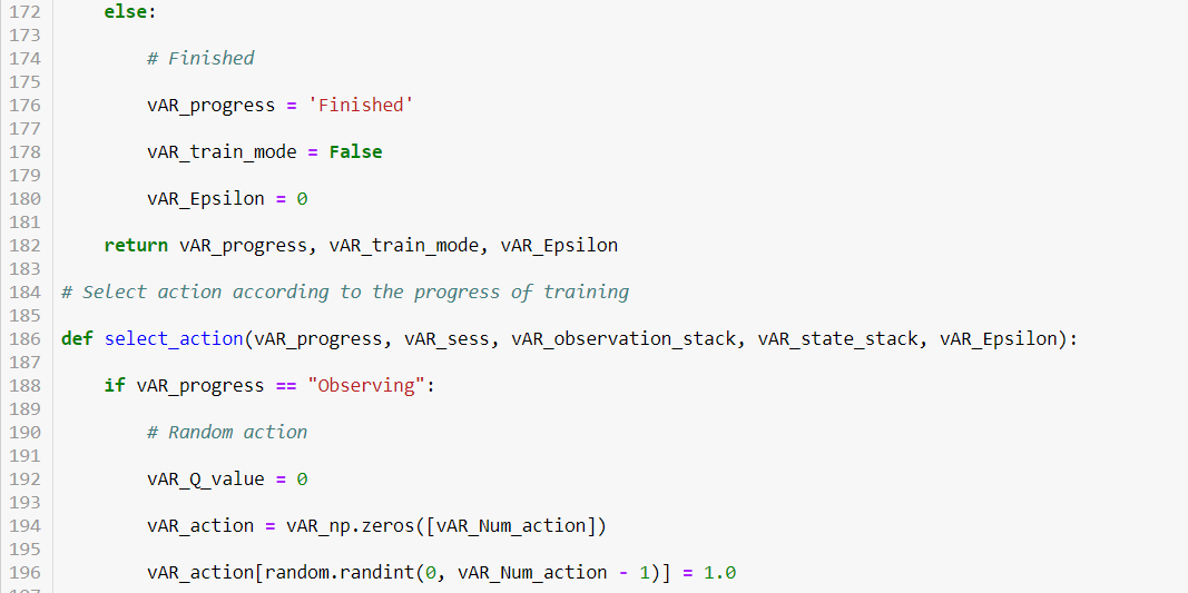
  • # Step 8 – Testing the Agent
    # Testing
    vAR_progress = 'Testing'
    vAR_train_mode = False
    vAR_Epsilon = 0
    else:
    # Finished
    vAR_progress = 'Finished'
    vAR_train_mode = False
    vAR_Epsilon = 0
    return vAR_progress, vAR_train_mode, vAR_Epsilon
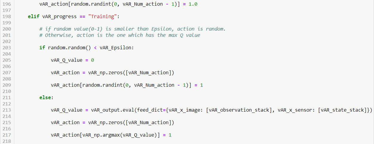
    # Select action according to the progress of training
    def select_action(vAR_progress, vAR_sess, vAR_observation_stack, vAR_state_stack, vAR_Epsilon):
    if vAR_progress == "Observing":
    # Random action
    vAR_Q_value = 0
    vAR_action = vAR_np.zeros([vAR_Num_action])
    vAR_action[random.randint(0, vAR_Num_action - 1)] = 1.0
    elif vAR_progress == "Training":
    # if random value(0-1) is smaller than Epsilon, action is random.
    # Otherwise, action is the one which has the max Q value
    if random.random() < vAR_Epsilon:
    vAR_Q_value = 0
    vAR_action = vAR_np.zeros([vAR_Num_action])
    vAR_action[random.randint(0, vAR_Num_action - 1)] = 1
    else:
    vAR_Q_value = vAR_output.eval(feed_dict={vAR_x_image: [vAR_observation_stack], vAR_x_sensor: [vAR_state_stack]})
    vAR_action = vAR_np.zeros([vAR_Num_action])
    vAR_action[vAR_np.argmax(vAR_Q_value)] = 1
    else:
    # Max Q action
    vAR_Q_value = vAR_output.eval(feed_dict={vAR_x_image: [vAR_observation_stack], vAR_x_sensor: [vAR_state_stack]})
    vAR_action = vAR_np.zeros([Num_action])
    vAR_action[vAR_np.argmax(Q_value)] = 1
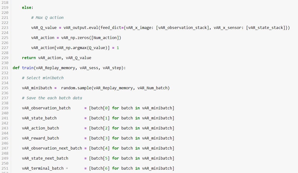
    return vAR_action, vAR_Q_value
    def train(vAR_Replay_memory, vAR_sess, vAR_step):
    # Select minibatch
    vAR_minibatch = random.sample(vAR_Replay_memory, vAR_Num_batch)
    # Save the each batch data
    vAR_observation_batch = [batch[0] for batch in vAR_minibatch]
    vAR_state_batch = [batch[1] for batch in vAR_minibatch]
    vAR_action_batch = [batch[2] for batch in vAR_minibatch]
    vAR_reward_batch = [batch[3] for batch in vAR_minibatch]
    vAR_observation_next_batch = [batch[4] for batch in vAR_minibatch]
    vAR_state_next_batch = [batch[5] for batch in vAR_minibatch]
    vAR_terminal_batch = [batch[6] for batch in vAR_minibatch]
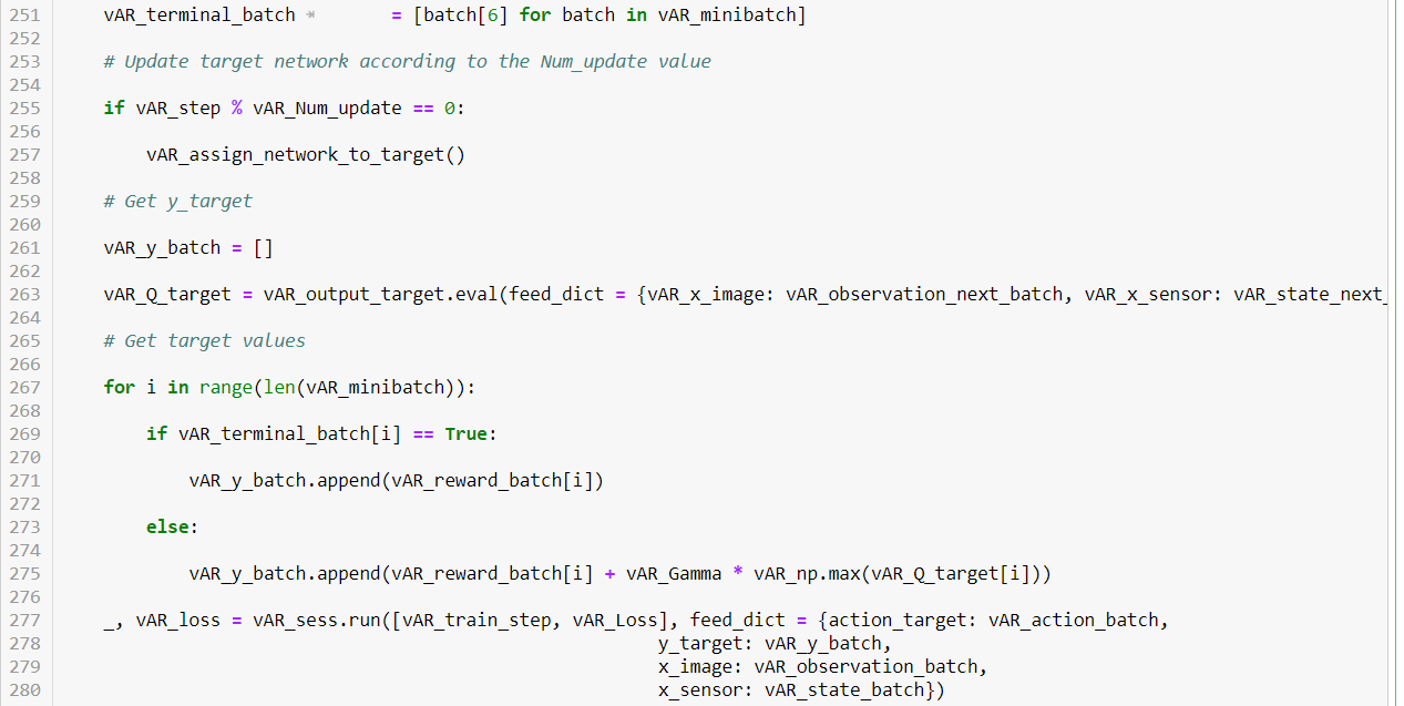
    # Update target network according to the Num_update value
    if vAR_step % vAR_Num_update == 0:
    vAR_assign_network_to_target()
    # Get y_target
    vAR_y_batch = []
    vAR_Q_target = vAR_output_target.eval(feed_dict = {vAR_x_image: vAR_observation_next_batch, vAR_x_sensor: vAR_state_next_batch})
    # Get target values
    for i in range(len(vAR_minibatch)):
    if vAR_terminal_batch[i] == True:
    vAR_y_batch.append(vAR_reward_batch[i])
    else:
    vAR_y_batch.append(vAR_reward_batch[i] + vAR_Gamma * vAR_np.max(vAR_Q_target[i]))
    _, vAR_loss = vAR_sess.run([vAR_train_step, vAR_Loss], feed_dict = {action_target: vAR_action_batch,
    y_target: vAR_y_batch,
    x_image: vAR_observation_batch,
    x_sensor: vAR_state_batch})
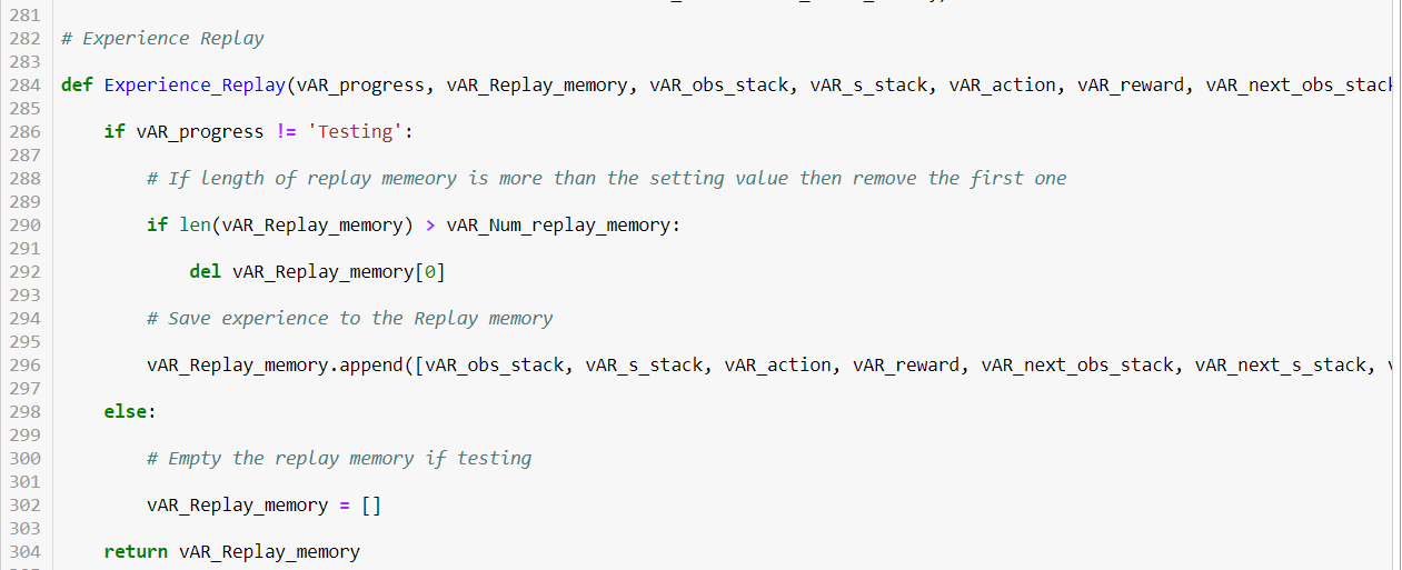
    # Experience Replay
    def Experience_Replay(vAR_progress, vAR_Replay_memory, vAR_obs_stack, vAR_s_stack, vAR_action, vAR_reward, vAR_next_obs_stack, vAR_next_s_stack, vAR_terminal):
    if vAR_progress != 'Testing':
    # If length of replay memeory is more than the setting value then remove the first one
    if len(vAR_Replay_memory) > vAR_Num_replay_memory:
    del vAR_Replay_memory[0]
    # Save experience to the Replay memory
    vAR_Replay_memory.append([vAR_obs_stack, vAR_s_stack, vAR_action, vAR_reward, vAR_next_obs_stack, vAR_next_s_stack, vAR_terminal])
    else:
    # Empty the replay memory if testing
    vAR_Replay_memory = []
    return vAR_Replay_memory
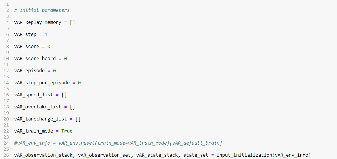
    # Initial parameters
    vAR_Replay_memory = []
    vAR_step = 1
    vAR_score = 0
    vAR_score_board = 0
    vAR_episode = 0
    vAR_step_per_episode = 0
    vAR_speed_list = []
    vAR_overtake_list = []
    vAR_lanechange_list = []
    vAR_train_mode = True
    #vAR_env_info = vAR_env.reset(train_mode=vAR_train_mode)[vAR_default_brain]
    vAR_observation_stack, vAR_observation_set, vAR_state_stack, state_set = input_initialization(vAR_env_info)
    vAR_check_plot = 0
    # Training & Testing
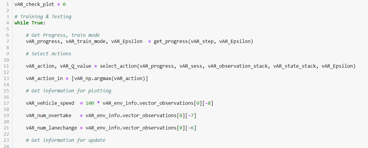
    while True:
    # Get Progress, train mode
    vAR_progress, vAR_train_mode, vAR_Epsilon = get_progress(vAR_step, vAR_Epsilon)
    # Select Actions
    vAR_action, vAR_Q_value = select_action(vAR_progress, vAR_sess, vAR_observation_stack, vAR_state_stack, vAR_Epsilon)
    vAR_action_in = [vAR_np.argmax(vAR_action)]
    # Get information for plotting
    vAR_vehicle_speed = 100 * vAR_env_info.vector_observations[0][-8]
    vAR_num_overtake = vAR_env_info.vector_observations[0][-7]
    vAR_num_lanechange = vAR_env_info.vector_observations[0][-6]
    # Get information for update
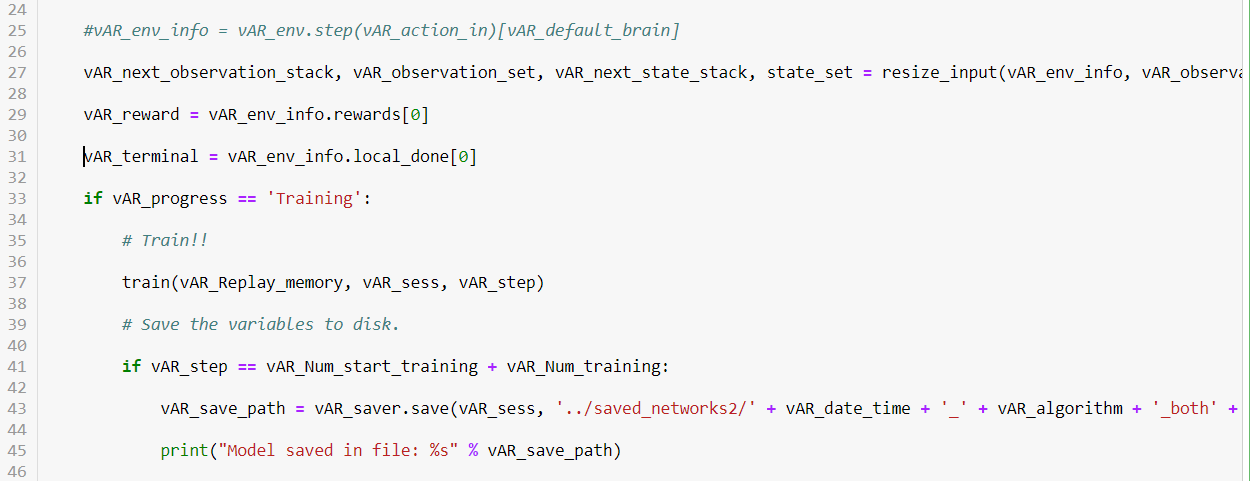
    #vAR_env_info = vAR_env.step(vAR_action_in)[vAR_default_brain]
    vAR_next_observation_stack, vAR_observation_set, vAR_next_state_stack, state_set = resize_input(vAR_env_info, vAR_observation_set, state_set)
    vAR_reward = vAR_env_info.rewards[0]
    vAR_terminal = vAR_env_info.local_done[0]
    if vAR_progress == 'Training':
    # Train!!
    train(vAR_Replay_memory, vAR_sess, vAR_step)
    # Save the variables to disk.
    if vAR_step == vAR_Num_start_training + vAR_Num_training:
    vAR_save_path = vAR_saver.save(vAR_sess, '../saved_networks2/' + vAR_date_time + '_' + vAR_algorithm + '_both' + "/model.ckpt")
    print("Model saved in file: %s" % vAR_save_path)
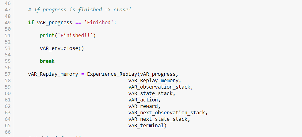
    # If progress is finished -> close!
    if vAR_progress == 'Finished':
    print('Finished!!')
    vAR_env.close()
    break
    vAR_Replay_memory = Experience_Replay(vAR_progress,
    vAR_Replay_memory,
    vAR_observation_stack,
    vAR_state_stack,
    vAR_action,
    vAR_reward,
    vAR_next_observation_stack,
    vAR_next_state_stack,
    vAR_terminal)
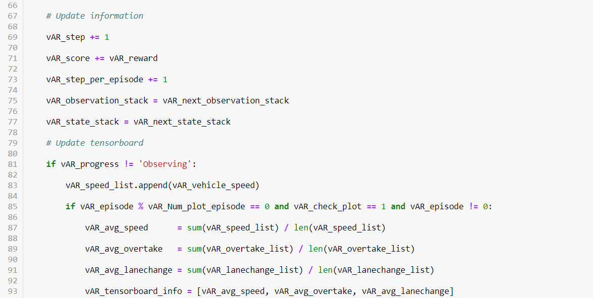
    # Update information
    vAR_step += 1
    vAR_score += vAR_reward
    vAR_step_per_episode += 1
    vAR_observation_stack = vAR_next_observation_stack
    vAR_state_stack = vAR_next_state_stack
    # Update tensorboard
    if vAR_progress != 'Observing':
    vAR_speed_list.append(vAR_vehicle_speed)
    if vAR_episode % vAR_Num_plot_episode == 0 and vAR_check_plot == 1 and vAR_episode != 0:
    vAR_avg_speed = sum(vAR_speed_list) / len(vAR_speed_list)
    vAR_avg_overtake = sum(vAR_overtake_list) / len(vAR_overtake_list)
    vAR_avg_lanechange = sum(vAR_lanechange_list) / len(vAR_lanechange_list)
    vAR_tensorboard_info = [vAR_avg_speed, vAR_avg_overtake, vAR_avg_lanechange]
    for i in range(len(vAR_tensorboard_info)):
    vAR_sess.run(update_ops[i], feed_dict = {summary_placeholders[i]: float(vAR_tensorboard_info[i])})
    vAR_summary_str = vAR_sess.run(vAR_summary_op)
    vAR_summary_writer.add_summary(vAR_summary_str, vAR_step)
    vAR_score_board = 0
    vAR_speed_list = []
    vAR_overtake_list = []
    vAR_lanechange_list = []
    vAR_check_plot = 0
    # If terminal is True
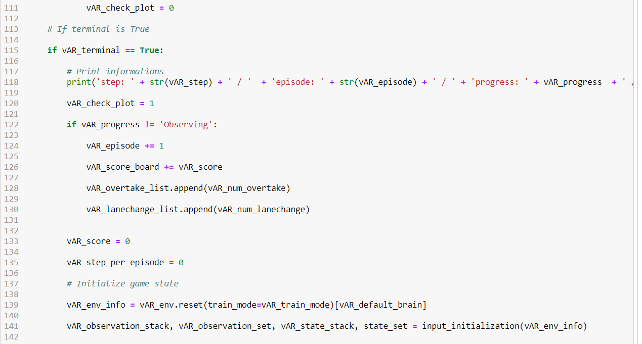
    if vAR_terminal == True:
    # Print informations
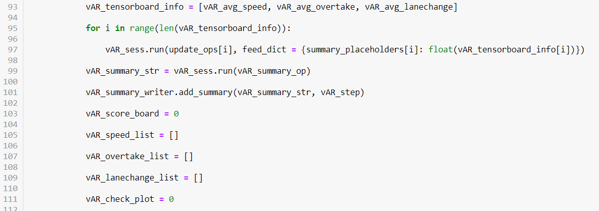
    print('step: ' + str(vAR_step) + ' / ' + 'episode: ' + str(vAR_episode) + ' / ' + 'progress: ' + vAR_progress + ' / ' + 'epsilon: ' + str(vAR_Epsilon) +' / ' + 'score: ' + str(vAR_score))
    vAR_check_plot = 1
    if vAR_progress != 'Observing':
    vAR_episode += 1
    vAR_score_board += vAR_score
    vAR_overtake_list.append(vAR_num_overtake)
    vAR_lanechange_list.append(vAR_num_lanechange)
    vAR_score = 0
    vAR_step_per_episode = 0
    # Initialize game state
    vAR_env_info = vAR_env.reset(train_mode=vAR_train_mode)[vAR_default_brain]
    vAR_observation_stack, vAR_observation_set, vAR_state_stack, state_set = input_initialization(vAR_env_info)
  • # Step 9 – Visually Test the Agent on the Environment
    ## Visually Test the Agent for Action & States on the Trained Environment
Model Implementation Steps

Step 0: Open Jupyter Notebook

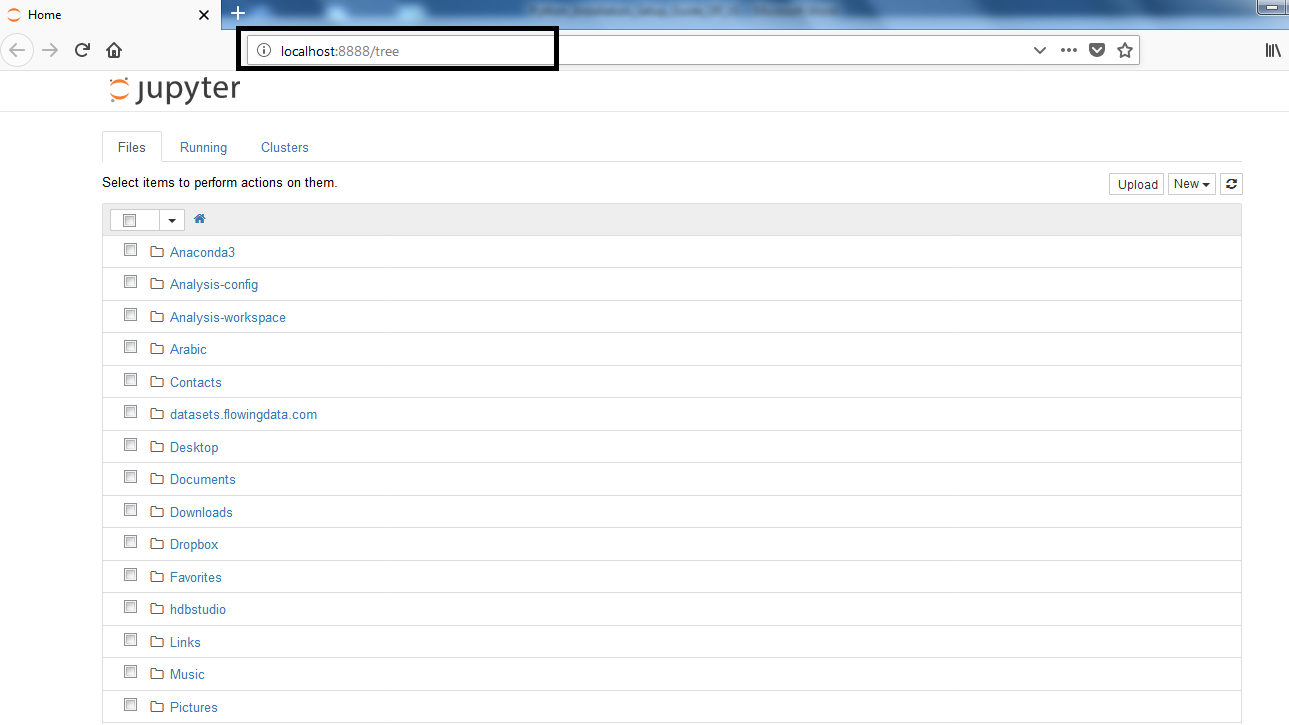
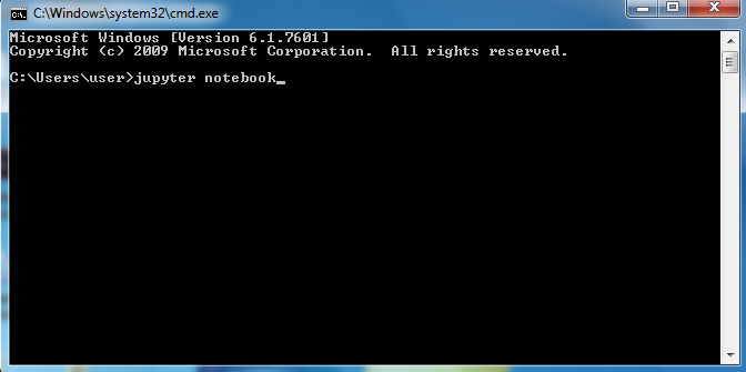
Jupiter notebook is launched through the command prompt. Type cmd & Search to Open Command prompt Terminal.
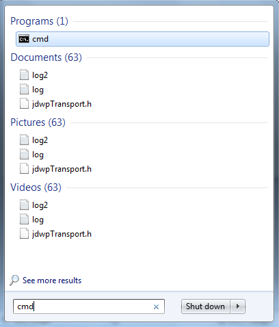
Model Implementation Steps

Now, Type Jupiter notebook & press Enter as shown
Model Implementation Steps

After typing, the Below Page opens

Model Implementation Steps

Open a New File or New Program in Jupyter Notebook

To Open a New File, follow the Below Instructions

Go to New >>> Python [conda root]

Model Implementation Steps

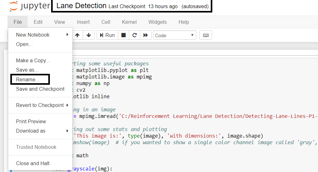
Give a meaningful name to the File as shown below.
Model Implementation Steps

Model Implementation Steps

Step 1- Import Required Libraries Used

For our Model Implementation we need the Following Libraries:

OpenCV: OpenCV is the leading open source library for computer vision, image processing and machine learning, and features GPU acceleration for real-time operation. Written in optimized C/C++, the library can take advantage of multi-core processing.

Numpy : NumPy is a general-purpose array-processing package. It provides a high-performance multidimensional array object, and tools for working with these arrays. It is the fundamental package for scientific computing with Python. It contains various features including these important ones:

  • A powerful N-dimensional array object
  • Sophisticated (broadcasting) functions
  • Tools for integrating C/C++ and Fortran code
  • Useful linear algebra, Fourier transform, and random number capabilities

Matplotlib : Matplotlib is a visualization library in Python for 2D plots of arrays. Matplotlib is a multi-platform data visualization library built on NumPy arrays and designed to work with the broader SciPy stack. It has greatest benefits of visualization is that it allows us visual access to huge amounts of data in easily digestible visuals.

Deep Neural Networks : A deep neural network is a neural network with a certain level of complexity, a neural network with more than two layers. Deep neural networks use sophisticated mathematical modeling to process data in complex ways. A neural network, in general, is a technology built to simulate the activity of the human brain specifically, pattern recognition and the passage of input through various layers of simulated neural connections.

Deep neural networks are networks that have an input layer, an output layer and at least one hidden layer in between. Each layer performs specific types of sorting and ordering in a process that some refer to as “feature hierarchy.” One of the key uses of these sophisticated neural networks is dealing with unlabelled or unstructured data. The phrase “deep learning” is also used to describe these deep neural networks, as deep learning represents a specific form of machine learning where technologies using aspects of artificial intelligence seek to classify and order information in ways that go beyond simple input/output protocols.

Deep Q-Networks : Deep Learning combined with Q-Learning yields Deep Q-Networks. In Deep Q-learning, we use a neural network to approximate the Q-value function. The state is given as the input and the Q-value of all possible actions is generated as the output.

Deep Q-Networks

It follows the below steps:

  1. All the past experience is stored by the user in memory
  2. The next action is determined by the maximum output of the Q-network.
  3. The loss function here is mean squared error of the predicted Q-value and the target Q-value Q*. This is basically a regression problem. However, we do not know the target or actual value here as we are dealing with a reinforcement learning problem.
Deep Q-Networks

Step 2 - Import the Input Data

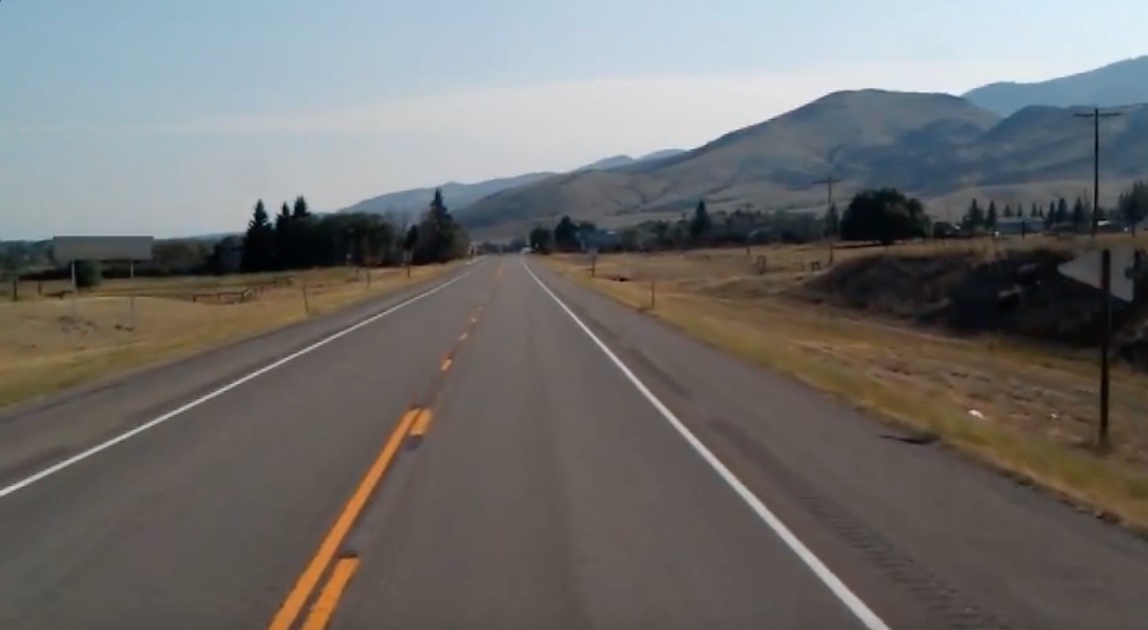
The input data is the Road Image from the Camera fixed in the Self-Driving Car. There are Several Cameras fixed inside the Self-Driving Car that captures the images & videos which act as input to the computer vision libraries used in our implementation:

Import the Input Data

Import the Input Data

Step 3 – Applying Various CV Techniques on the Input Camera Image

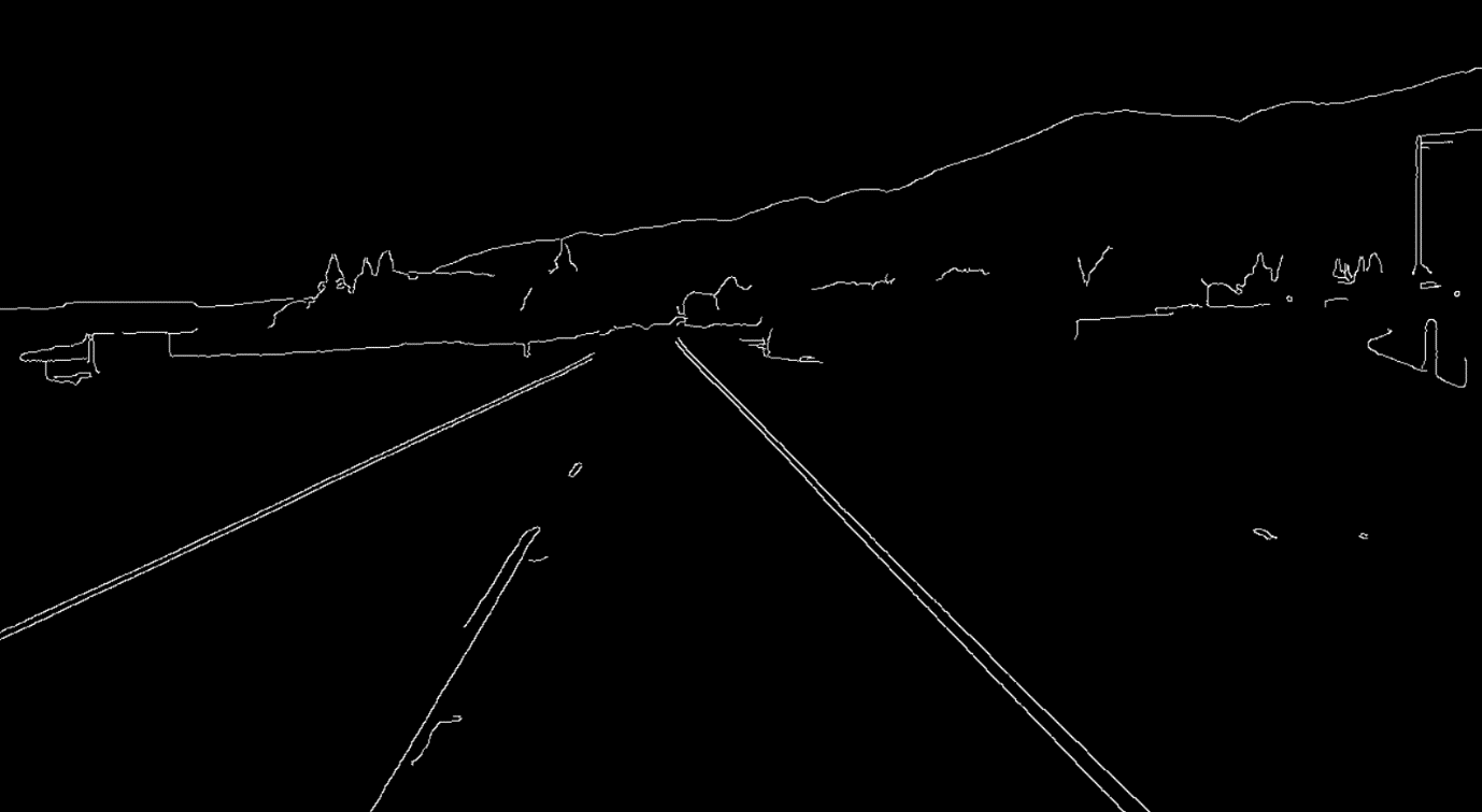
Canny Edge Detection: Canny Edge Detection uses a multi-stage algorithm to detect a wide range of edges in images. Edge detection is an essential image analysis technique when someone is interested in recognizing objects by their outlines, and is also considered an essential step in recovering information from images. For instance, important features like lines and curves can be extracted using edge detection, which are then normally used by higher-level computer vision or image processing algorithms. A good edge detection algorithm would highlight the locations of major edges in an image, while at the same time ignoring any false edges caused by noise.

Canny Edge Detection involves series of steps
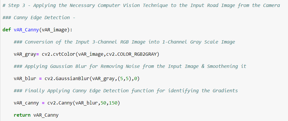
  • Converting the 3-Channel RGB into 1-Channel gray scale image
  • Applying Gaussian Blur on the converted gray scale image for noise reduction & smoothing
  • Finally Apply Canny edge detector on the gaussian blurred image
Canny Edge Detection

Canny Edge Detection

Region of Interest: Region of interest focusses on only the area that is in the interest of lane detection. With that in view a polygon is drawn with fillpoly function.
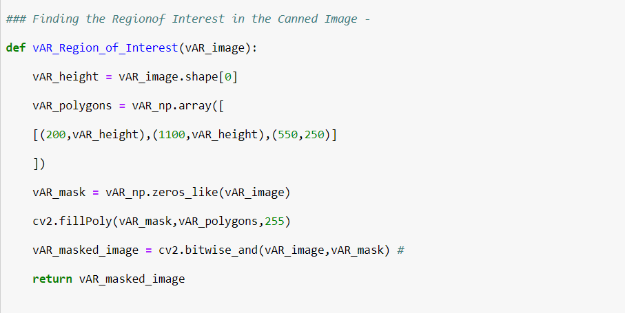
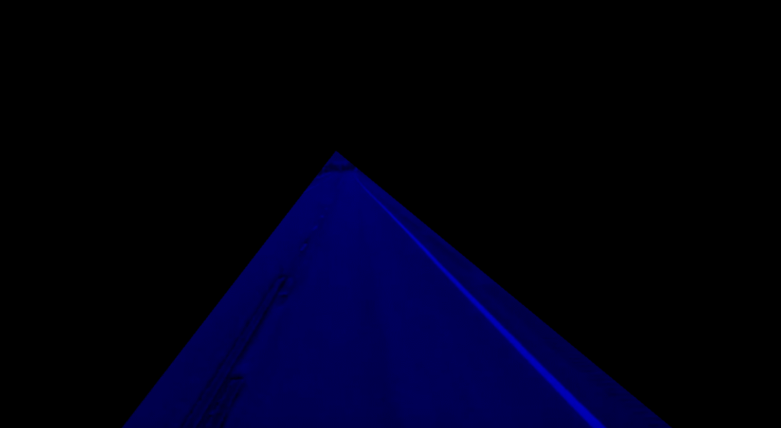
Region of Interest

Region of Interest

Hough Transform: The Hough transform is a feature extraction technique used in image analysis, computer vision. The Hough transform is concerned with the identification of lines in the image, then the Hough transform has been extended to identifying positions of arbitrary shapes, most commonly circles or ellipses. Here in our Implementation it is used for feature extraction in the masked image. Since the area concerned with the region interest is an vector space with features & labels, it can be used to draw a straight line along the lane markings.
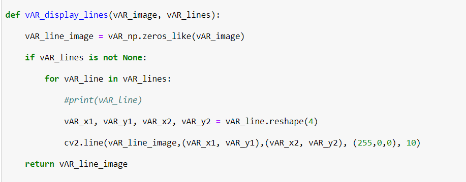
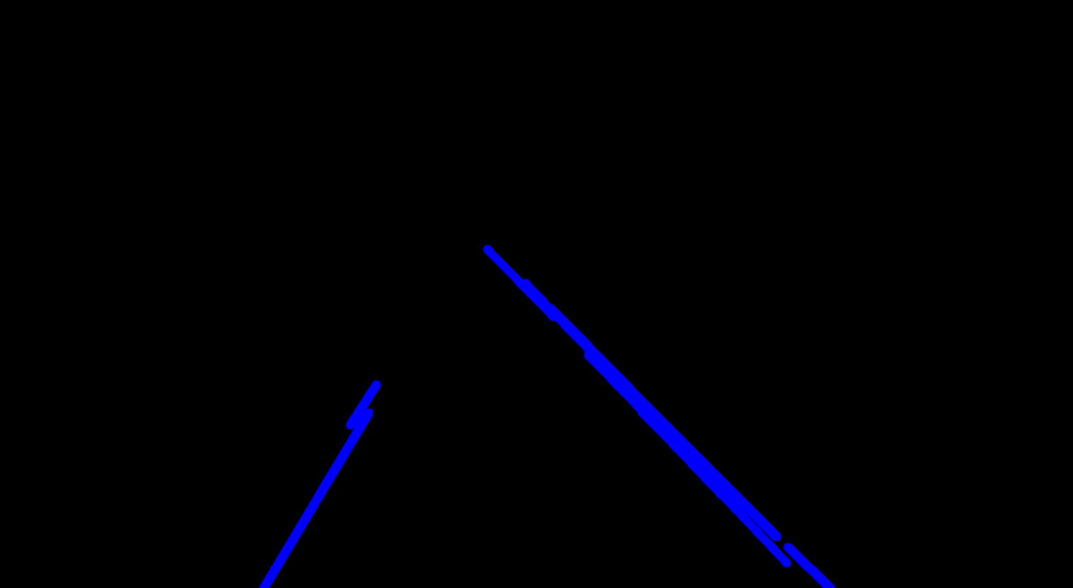
Hough Transform

Hough Transform

Original Road Image with lane Detection
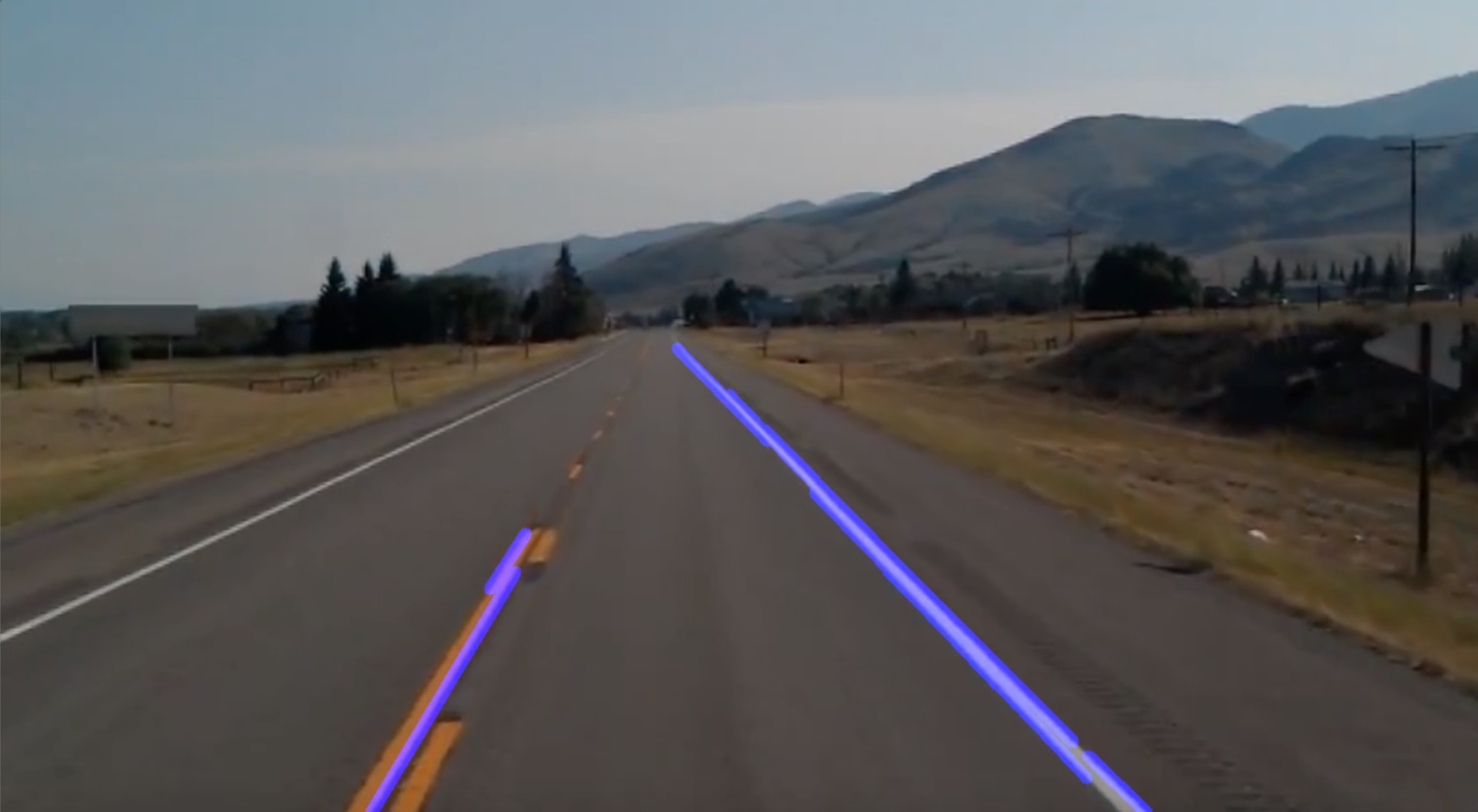
Road Image with lane Detection

Road Image with lane Detection
The Overall Process that an Input Road Image Undergoes

Step 4 – Downloading the Environment & Installing the Agents

Downloading the Environment:: The Environment is typically a set of states the "agent" is attempting to influence via its choice of "actions". The agent arrives at different scenarios known as states by performing actions. Actions lead to rewards which could be positive and negative.

Downloading the Environment & Installing the Agents
A Typical Agent - Environment Setup

The Environment we are using in this Implementation is an Unity Self driven car Environment that can be downloaded from the below link: https://www.dropbox.com/s/7xti37jv3d28u1z/environment_windows.zip?dl=0

After the Environment is downloaded, Clone the Self Driven Car Repository from the below Link. https://github.com/MLJejuCamp2017/DRL_based_SelfDrivingCarControl

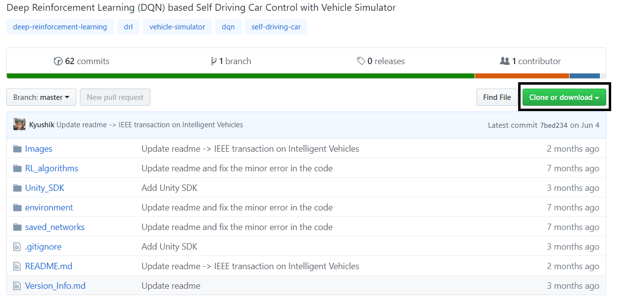
Downloading the Environment & Installing the Agents

Downloading the Environment & Installing the Agents

After you clone or download the self-driven car repo, copy & paste all the files from the environment folder (Downloaded from the dropbox) into the environment folder of the cloned repository as shown (First unzip the downloaded folder):
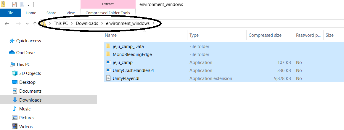
Downloading the Environment & Installing the Agents
Environment Binary files downloaded from the dropbox

Downloading the Environment & Installing the Agents
Copy & paste all the files into the environment folder

Downloading the Agents

In Our implementation we will be using Unity ML-Agents Toolkit.The Unity Machine Learning Agents Toolkit (ML-Agents) is an open-source Unity plugin that enables games and simulations to serve as environments for training intelligent agents. Agents can be trained using reinforcement learning, imitation learning, neuroevolution, or other machine learning methods through a simple-to-use Python API. The ML-Agents toolkit is mutually beneficial for both game developers and AI researchers as it provides a central platform where advances in AI can be evaluated on Unity’s rich environments and then made accessible to the wider research and game developer communities.

Following are the features of ML-agents toolkit

  • Unity environment control from Python
  • Support for multiple environment configurations and training scenarios
  • Train memory-enhanced agents using deep reinforcement learning
  • Easily definable Curriculum Learning and Generalization scenarios
  • Broadcasting of agent behaviour for supervised learning
  • Built-in support for Imitation Learning
  • Flexible agent control with On Demand Decision Making
  • Visualizing network outputs within the environment
  • Simplified set-up with Docker
  • Wrap learning environments as a gym
  • Utilizes the Unity Inference Engine

The ML-Agents tool kit can be downloaded & install in two ways:

  1. Pip install from the PyPi python repository.
  2. Pip install from the cloned ml-agents repository.

To install and use ML-Agents, first you need to install Unity, clone this repository and install Python with additional dependencies

Install Unity 2017.4 or Later from the below link

https://store.unity.com/download

Downloading & Installing from the PyPi python Repository: The Python Package Index (PyPI) is a repository of software for the Python programming language. PyPI helps you find and install software developed and shared by the Python community. Use PyPi to install ML-Agents as shown below

Open Windows Command Prompt as shown
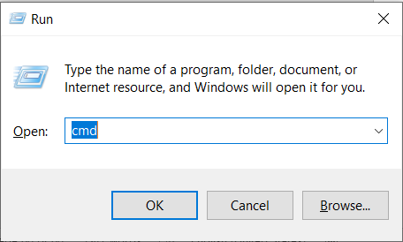
Downloading & Installing from the PyPi python Repository

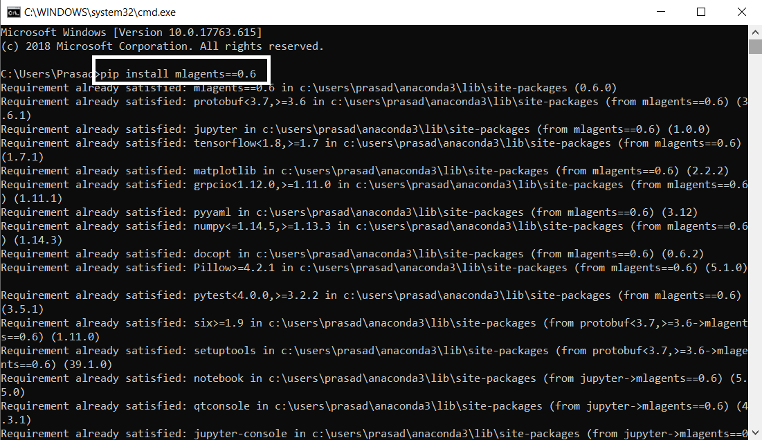
Once the Command Prompt window launches type pip install mlagents==0.6
Downloading & Installing from the PyPi python Repository

Note that pip install mlagents==0.6 will install ml-agents from PyPi, not from the cloned repo. If installed correctly, you should be able to run mlagents-learn --help, after which you will see the Unity logo and the command line parameters you can use with mlagents-learn.

By installing the mlagents package, the dependencies listed in the setup.py file are also installed. Some of the primary dependencies include:

  • TensorFlow (Requires a CPU w/ AVX support)
  • Jupyter

Downloading & Installing from the cloned ML-agents Repository:

To clone the ml-agents repository visit the below URL

Downloading & Installing from the cloned ML-agents Repository

If Git is already installed then using git clone the Repository as shown. If Git is not installed download & install Git from the below link

https://git-scm.com/downloads

Downloading & Installing from the cloned ML-agents Repository

Downloading & Installing from the cloned ML-agents Repository

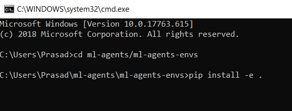
If you intend to make modifications to ml-agents or ml-agents-envs, you should install the packages from the cloned repo rather than from PyPi. To do this, you will need to install ml-agents and ml-agents-envs separately. Open windows command prompt, navigate to the Cloned repo's root directory as shown

Open Windows Command Prompt as shown

Downloading & Installing from the cloned ML-agents Repository

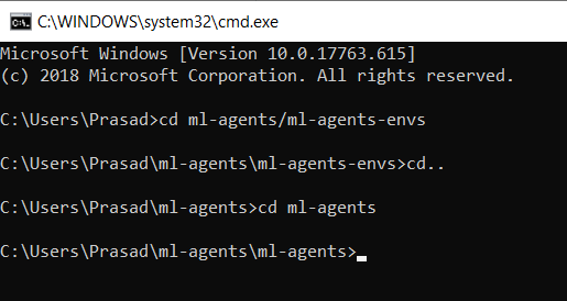
Navigate to the cloned repository root directory & then type cd ml-agents/ml-agents-envs
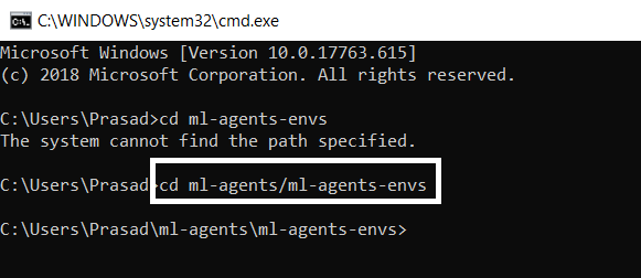
Downloading & Installing from the cloned ML-agents Repository

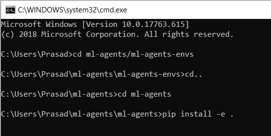
Type pip install -e .

Downloading & Installing from the cloned ML-agents Repository

After the Installation completes, type cd.. to navigate back to ml-agents folder
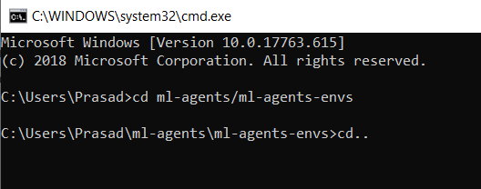
Downloading & Installing from the cloned ML-agents Repository

type cd ml-agents/ml-agents-envs

Downloading & Installing from the cloned ML-agents Repository

Type pip install -e .

Downloading & Installing from the cloned ML-agents Repository

Now that you have the environment both from unity & python end, start the environment, so that you can interact with the unity environment through python as shown

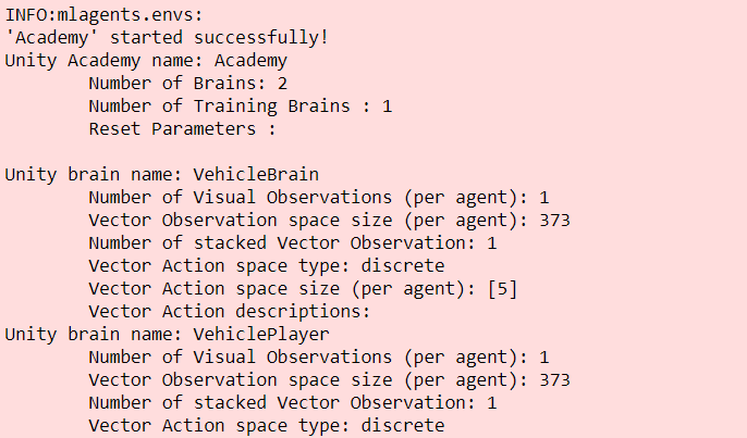
Environments contain brains which are responsible for deciding the actions of their associated agents. Here we check for the first brain available, and set it as the default brain we will be controlling from Python.

Downloading & Installing from the cloned ML-agents Repository

Step 5 – Examine the Observation & State Spaces

We can reset the environment to be provided with an initial set of observations and states for all the agents within the environment. In ML-Agents, states refer to a vector of variables correspondingto relevant aspects of the environment for an agent. Likewise, observations refer to a set of relevant pixel-wise visuals for an agent.
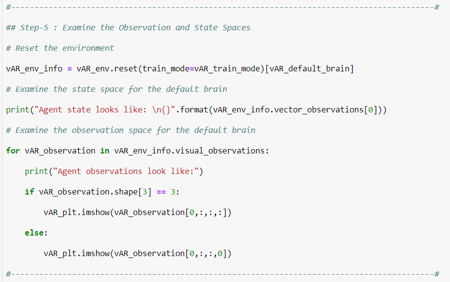
Examine the Observation & State Spaces

This is how the brain the looks like

Examine the Observation & State Spaces

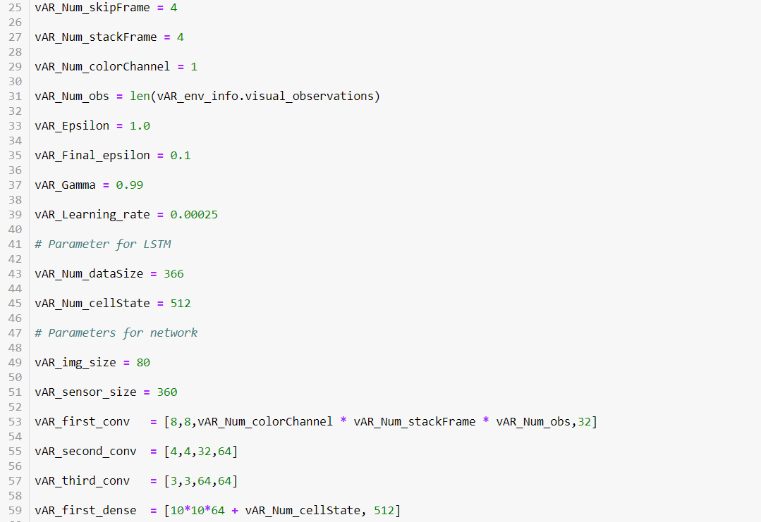
Step 6 – Build a Neural Network Architecture for DQN

In Deep Q-learning, we use a neural network to approximate the Q-value function. The state is given as the input and the Q-value of all possible actions is generated as the output.

Following are the steps involved in reinforcement learning using deep Q-learning networks (DQNs)?

  1. All the past experience is stored by the user in memory
  2. The next action is determined by the maximum output of the Q-network
  3. The loss function here is mean squared error of the predicted Q-value and the target Q-value – Q*. This is basically a regression problem. However, we do not know the target or actual value here as we are dealing with a reinforcement learning problem. Going back to the Q-value update equation derived from the Bellman equation. we have:
Build a Neural Network Architecture for DQN

Build a Neural Network Architecture for DQN

Build a Neural Network Architecture for DQN

Build a Neural Network Architecture for DQN

Build a Neural Network Architecture for DQN

Build a Neural Network Architecture for DQN

Build a Neural Network Architecture for DQN

Build a Neural Network Architecture for DQN

Build a Neural Network Architecture for DQN

Build a Neural Network Architecture for DQN

Build a Neural Network Architecture for DQN

Build a Neural Network Architecture for DQN

Build a Neural Network Architecture for DQN

Build a Neural Network Architecture for DQN

Step 7 – Training the Agent to Interact with the Environment

Train the Agent to interact with the environment. We can step the environment forward and provide actions to all of the agents within the environment. The Agent is trained for actions based on the action_space_type of the default brain.
Training the Agent to Interact with the Environment

Training the Agent to Interact with the Environment

Training the Agent to Interact with the Environment

Training the Agent to Interact with the Environment

Training the Agent to Interact with the Environment

Training the Agent to Interact with the Environment

Training the Agent to Interact with the Environment

Training the Agent to Interact with the Environment

Training the Agent to Interact with the Environment

Training the Agent to Interact with the Environment

Training the Agent to Interact with the Environment

Training the Agent to Interact with the Environment

Training the Agent to Interact with the Environment

Training the Agent to Interact with the Environment

Training the Agent to Interact with the Environment

Step 8 – Testing the Agent to Interact with the Environment

Testing the Agent to Interact with the Environment

Testing the Agent to Interact with the Environment

Testing the Agent to Interact with the Environment

Testing the Agent to Interact with the Environment

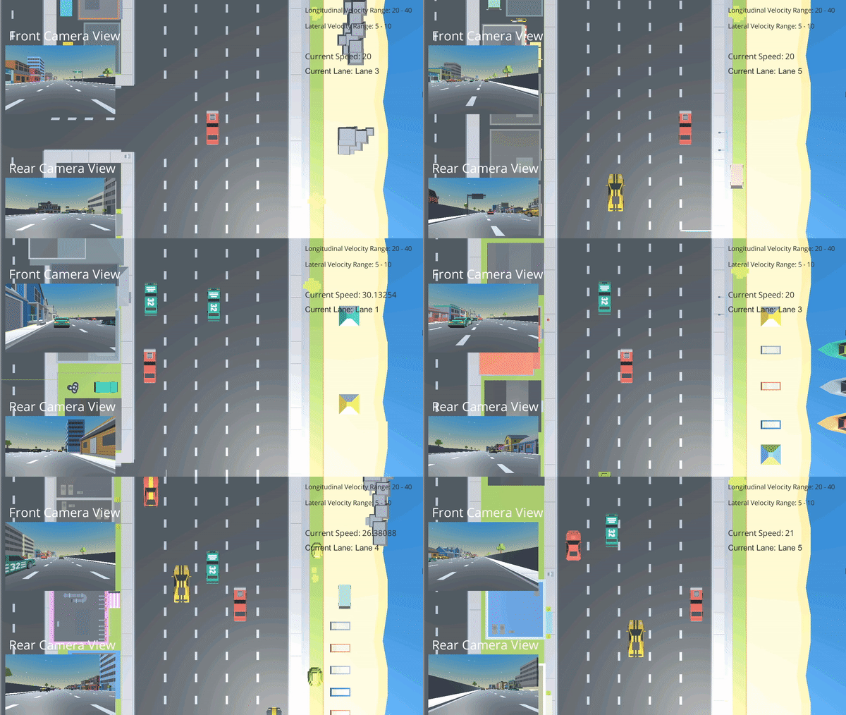
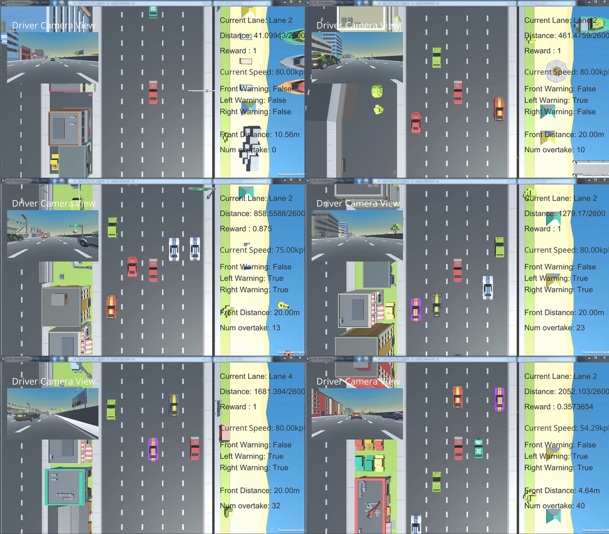
Step 9 – Testing the Self-driving car on for Lane Detection & Changes

Before Training

Testing the Self-driving car on for Lane Detection & Changes

After Training

Testing the Self-driving car on for Lane Detection & Changes

Conclusion

In this lab work, we have used Deep Q Networks, a reinforcement learning model to train the self-driving car environment on the agent. The model performed well on the & was able to produce the outcome as expected.

This is an implementation to learn and better understand the overall steps and processes that are involved in implementing a reinforcement learning model. There are a lot more steps, processes, data and technologies involved. We strongly request and recommend you to learn and prepare yourself to address real-world problems.

Customers’ Vocal Endorsements
We have been delivering impactable products and services on artificial intelligence, data engineering, finance, analytics, training and talent development for every business function. We work closely with senior executives as well as technical developers.


Download Request
Contact

Point of Contact

Jothi Periasamy
Chief AI Architect


Address

2100 Geng Road
Suite 210
Palo Alto
CA 94303


Contact e-Mail

lnfo@DeepSphere.AI


Contact Phone

(916)-296-0228


Web

https://www.deepsphere.ai

Join our Newsletter list to get all the latest articles, posts and other benefits